SVM in Machine Learning: A Beginner’s Guide
Feb 12, 2026 5 Min Read 3117 Views
(Last Updated)
Wondering what SVM is and why it sounds so complicated? Well, Support Vector Machine (SVM) in machine learning stands as one of the most powerful yet flexible supervised algorithms you can master for classification and regression tasks.
Support Vector Machines (SVM) work by creating an optimal hyperplane that maximizes the margin between different classes. This approach effectively separates data points while maintaining the highest possible distance from the closest points (known as support vectors). It’s not easy to understand as a beginner, but I’m here to help.
Throughout this beginner’s guide, you’ll learn what SVMs are, how they function, and why they remain relevant in today’s machine learning landscape. We’ll break down complex concepts into simple explanations and show you how to get started with SVM implementations. Let’s begin!
Table of contents
- What is SVM in Machine Learning?
- Why is SVM used in machine learning
- Common use cases for SVM
- How Does SVM Work?
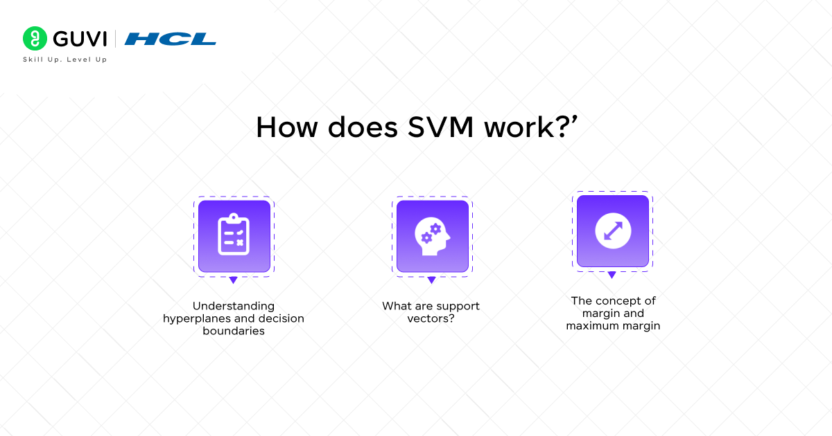
- 1) Understanding hyperplanes and decision boundaries
- 2) What are support vectors?
- 3) The concept of margin and maximum margin
- Linear vs Non-Linear SVM
- 1) Core Idea
- 2) Key Differences
- 3) When to Use Linear SVM
- 4) What is Non-Linear SVM?
- 5) Use Case Examples
- Implementing SVM in Python
- 1) Using scikit-learn for SVM
- 2) Working with the Iris dataset
- 3) Visualizing decision boundaries
- 4) Tuning parameters like C and gamma
- Concluding Thoughts…
- FAQs
- Q1. What is SVM and how does it work in machine learning?
- Q2. When should I use linear SVM versus non-linear SVM?
- Q3. What is the kernel trick in SVM?
- Q5. What are the key parameters to tune in SVM?
What is SVM in Machine Learning?
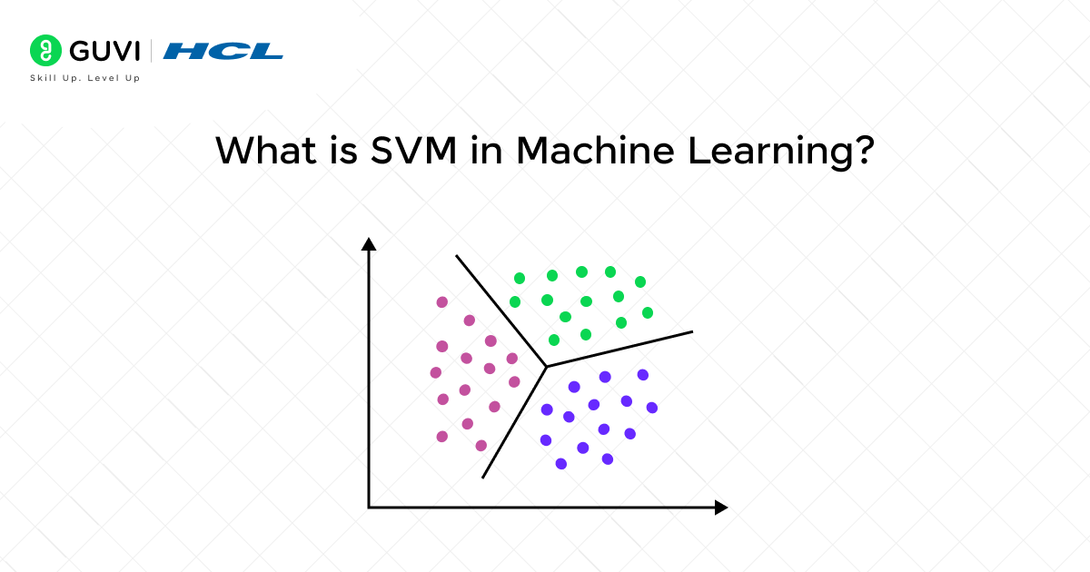
A Support Vector Machine (SVM) is a powerful supervised machine learning algorithm designed for classification, regression, and outlier detection tasks. This algorithm works by finding the optimal hyperplane (a decision boundary) that effectively separates data points of different classes. The main goal is to maximize the margin—the distance between this boundary and the closest data points from each class.
Why is SVM used in machine learning
SVMs have gained popularity in the machine learning community for several compelling reasons:
- Effectiveness with complex data – SVMs perform exceptionally well in high-dimensional spaces and remain effective even when the number of dimensions exceeds the number of samples.
- Memory efficiency – Instead of using the entire dataset, SVMs only use a subset of training points (called support vectors) in their decision function, making them memory-efficient.
- Versatility – Through the “kernel trick,” SVMs can handle both linear and non-linear classification problems by transforming data into higher dimensions where it becomes more easily separable.
- Robustness – SVMs are less prone to overfitting, particularly in high-dimensional spaces, thanks to their regularization parameters.
- Accuracy – For smaller datasets, especially where dimensions outnumber samples, SVMs provide highly accurate results.
Furthermore, SVMs offer clear interpretability with their decision boundaries, making them valuable for understanding model predictions and making informed decisions.
Common use cases for SVM
SVMs are widely used due to their ability to handle high-dimensional and complex data. Key applications include:
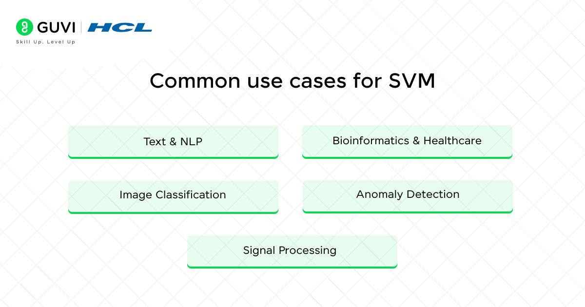
- Text & NLP: Spam detection, sentiment analysis, topic classification—ideal for handling sparse, high-dimensional text data.
- Image Classification: Effective in facial recognition, object detection, and handwriting analysis; often outperforms traditional methods.
- Bioinformatics & Healthcare: Used in gene expression analysis, protein classification, and cancer detection; achieves up to 96–97% accuracy in seismic ground strength prediction.
- Anomaly Detection: One-class SVMs help identify outliers in fraud detection and cybersecurity.
- Signal Processing: Applied in speech recognition and biomedical signal interpretation.
How Does SVM Work?
At its core, Support Vector Machine (SVM) operates by constructing an optimal hyperplane to separate data points belonging to different classes. The mechanism behind SVM focuses on finding the best possible decision boundary that maximizes the distance between classes, thereby creating a robust classification model.
1) Understanding hyperplanes and decision boundaries
In the SVM framework, a hyperplane serves as the decision boundary that divides your data into distinct categories. In simple terms, a hyperplane in a two-dimensional space is simply a line, while in three dimensions, it becomes a plane. For higher dimensions, it’s a (d-1)-dimensional subspace within a d-dimensional space.
The mathematical representation of a hyperplane is: w·x + b = 0
Where:
- w represents the weight vector perpendicular to the hyperplane
- x is the input feature vector
- b is the bias term
For a given data point, the sign of the function w·x + b determines its class. If the result is positive, the point belongs to one class; if negative, it belongs to the other. Essentially, this creates a clear division between different categories in your dataset.
2) What are support vectors?
Support vectors are the critical data points that lie closest to the decision boundary. These points are fundamentally important because:
- They directly determine the position and orientation of the hyperplane
- They’re the most challenging samples to classify
- They’re the only data points needed to define the decision function
Unlike other machine learning algorithms that use all training data points to build a model, SVM only utilizes these support vectors in its decision function, making it memory-efficient. Moreover, the optimization algorithm generates weights in such a way that only the support vectors influence the boundary.
3) The concept of margin and maximum margin
The margin in SVM refers to the distance between the hyperplane and the closest data points (support vectors) from each class. Mathematically, this margin equals 2/||w||, where ||w|| is the norm of the weight vector.
SVM strives to maximize this margin because:
- A larger margin typically results in better generalization to unseen data
- It reduces the risk of overfitting
- It creates a more robust model that’s less sensitive to small changes in the data
The optimal hyperplane is the one that achieves the maximum possible margin between classes while correctly classifying the training points. This maximum-margin classifier is what gives SVM its power and effectiveness in various classification tasks.
Linear vs Non-Linear SVM
Understanding the difference between linear and non-linear Support Vector Machines (SVMs) is crucial for choosing the right approach for your classification tasks. Let’s explore these two fundamental types of SVMs and when to use each.
1) Core Idea
- A Linear SVM tries to separate classes using a straight line (in 2D) or a flat surface (in higher dimensions).
- A Non-Linear SVM can create curved or complex boundaries to separate data that can’t be split using a straight line.
2) Key Differences
| Aspect | Linear SVM | Non-Linear SVM |
| Decision Boundary | Straight line (2D) or flat hyperplane | Curved or complex surface |
| When It Works Best | When data is linearly separable | When data follows non-linear patterns |
| Speed and Simplicity | Fast, easy to train, interpretable | Slower, more complex to train |
| Computational Cost | Low (efficient for large or sparse datasets) | Higher (requires kernel computations) |
| Interpretability | Easy to understand and explain | Harder to visualize and interpret |
| Common Kernels Used | Not needed (uses raw features) | RBF, Polynomial, Sigmoid (to transform input space) |
3) When to Use Linear SVM
Use Linear SVM if:
- Your dataset is linearly separable – a single line or plane can divide the classes.
- You’re working with high-dimensional data, such as text classification.
- You need a simple, fast, and interpretable model.
- You’re dealing with large datasets or have limited computational resources.
Examples:
- Spam vs. non-spam email classification
- Sentiment analysis on product reviews
- Document topic classification
4) What is Non-Linear SVM?
When data has complex patterns, Non-Linear SVMs can help. They use something called the kernel trick to map the data into a higher-dimensional space, where it becomes linearly separable.
Common Kernels:
- RBF (Radial Basis Function): Ideal for circular or radial class distributions.
- Polynomial: Captures more complex, curved boundaries.
These kernels let SVMs draw flexible, non-linear boundaries in the original feature space.
5) Use Case Examples
Non-Linear SVM is ideal when:
- Classes form clusters, rings, or complex shapes.
- You’re working on:
- Facial recognition
- Handwriting classification
- Medical diagnosis (e.g., cancer detection)
- Customer segmentation with overlapping features
Implementing SVM in Python
Getting hands-on with SVM requires practical implementation. Python’s scikit-learn library offers an excellent framework to experiment with support vector machines directly on real datasets.

1) Using scikit-learn for SVM
Scikit-learn makes implementing SVM remarkably straightforward through its well-designed API. To get started with SVM in Python:
from sklearn import svm
from sklearn.preprocessing import StandardScaler
# Create SVM classifier

clf = svm.SVC(kernel='linear')  # Linear kernel

# clf = svm.SVC(kernel='rbf')   # RBF kernel
The SVC class handles both binary and multi-class classification problems. Before training, data preprocessing is essential as SVMs are not scale-invariant. Use StandardScaler to normalize your features for optimal performance.
2) Working with the Iris dataset
The Iris dataset serves as an ideal starting point for SVM implementation:
from sklearn import datasets

iris = datasets.load_iris()

X = iris.data[:, :2]  # Using first two features

y = iris.target

# Split dataset into training and testing sets

from sklearn.model_selection import train_test_split

X_train, X_test, y_train, y_test = train_test_split(X, y, test_size=0.3)

# Train the model and predict

clf.fit(X_train, y_train)

predictions = clf.predict(X_test)
This classic dataset contains measurements of iris flowers and their corresponding species, making it perfect for classification tasks.
3) Visualizing decision boundaries
Visualizing SVM decision boundaries helps understand how your model separates classes:
import matplotlib.pyplot as plt

import numpy as np

# Create mesh grid

x_min, x_max = X[:, 0].min() - 1, X[:, 0].max() + 1

y_min, y_max = X[:, 1].min() - 1, X[:, 1].max() + 1

xx, yy = np.meshgrid(np.arange(x_min, x_max, 0.01),

                     np.arange(y_min, y_max, 0.01))

# Predict on mesh grid points

Z = clf.predict(np.c_[xx.ravel(), yy.ravel()])

Z = Z.reshape(xx.shape)

# Plot decision boundary

plt.contourf(xx, yy, Z, alpha=0.8)

plt.scatter(X[:, 0], X[:, 1], c=y, edgecolors='k')
This visualization technique creates a colored contour plot showing regions where the model predicts different classes.
4) Tuning parameters like C and gamma
The performance of SVM depends primarily on two critical parameters:
- C parameter: Controls the trade-off between smooth decision boundary and classifying training points correctly
- Lower C: Smoother decision boundary but may misclassify more points
- Higher C: Fewer misclassifications but potential overfitting
- Gamma parameter: Defines how far the influence of a single training example reaches
- Low gamma: Wider influence, smoother boundaries
- High gamma: More complex, potentially overfitted boundaries
For proper tuning, use GridSearchCV:
from sklearn.model_selection import GridSearchCV

param_grid = {'C': [0.1, 1, 10, 100], 'gamma': [0.1, 1, 10, 100]}

grid = GridSearchCV(svm.SVC(kernel='rbf'), param_grid, cv=5)

grid.fit(X_train, y_train)

print("Best parameters:", grid.best_params_)
This systematic approach finds the optimal parameter combination through cross-validation.
To dive deeper into concepts like SVM and master practical machine learning skills, check out HCL GUVI’s Artificial Intelligence and Machine Learning Course. Designed for beginners, it offers hands-on projects, industry-ready content, and mentorship from experts to fast-track your ML career.
Concluding Thoughts…
Support Vector Machines certainly stand as one of the most versatile algorithms in the machine learning toolkit. Throughout this guide, you’ve learned how SVMs create optimal decision boundaries by maximizing the margin between different classes. Additionally, you’ve discovered the power of the kernel trick that transforms complex non-linear problems into solvable linear ones.
What makes SVMs particularly valuable is their effectiveness with high-dimensional data while remaining computationally efficient by focusing only on support vectors. While SVMs might initially seem mathematically intimidating, the scikit-learn implementation makes these powerful algorithms accessible to beginners. With just a few lines of code, you can build robust classifiers that handle complex real-world problems.
As you continue your journey in data science, the principles behind SVMs will undoubtedly enhance your understanding of other classification techniques and help you build more effective models. Good Luck!
FAQs
Q1. What is SVM and how does it work in machine learning?
SVM (Support Vector Machine) is a supervised learning algorithm used for classification and regression tasks. It works by finding an optimal hyperplane that maximally separates different classes of data points, focusing on the closest points called support vectors to determine the decision boundary.
Q2. When should I use linear SVM versus non-linear SVM?
Use linear SVM when your data is linearly separable or when working with high-dimensional data like text classification. Non-linear SVM is better for complex, non-linearly separable data patterns, often using kernel functions to transform the data into higher dimensions where it becomes separable.
Q3. What is the kernel trick in SVM?
The kernel trick is a technique that allows SVMs to handle non-linear classification problems efficiently. It implicitly maps input data into higher-dimensional spaces where linear separation becomes possible, without actually computing the coordinates in that space, thus saving computational resources.
Q5. What are the key parameters to tune in SVM?
The two most critical parameters to tune in SVM are C and gamma. C controls the trade-off between having a smooth decision boundary and classifying training points correctly, while gamma defines how far the influence of a single training example reaches. These can be optimized using techniques like GridSearchCV in scikit-learn.








Did you enjoy this article?