Bayes’ Theorem in Machine Learning 2026: Complete Guide for ML Beginners

Bayes’ Theorem in machine learning is an unsung hero. It powers many smart systems you use every day. This includes your email’s spam filter, as well as it drives recommendation engines. Yet, few grasp how it learns from each new piece of evidence. 

Whether you are curious about Naive Bayes classifiers, Bayesian networks, or hierarchical models, this post will show you how to balance prior knowledge with fresh observations. Read the full blog to follow each step and learn how to apply Bayesian inference in your projects.

What is Bayes’ Theorem?

Bayes’ Theorem is a mathematical rule for updating probability when new evidence becomes available. It connects what you believed before seeing the evidence with what you should believe after observing it.

In machine learning, the theorem helps data scientists calculate an updated probability for a hypothesis based on observed data.

It originated from the work of Reverend Thomas Bayes in the 18th century. Today, the theorem forms a central part of Bayesian statistics and probabilistic machine learning.

Suppose a model initially estimates that an email has a 20% chance of being spam. It then detects words that frequently appear in spam messages. Bayes’ Theorem helps the model combine that new evidence with its original estimate and calculate an updated spam probability.

This process is based on four components:

• Prior probability: What you believe before observing new evidence.
• Likelihood: How probable the evidence is under a particular hypothesis.
• Evidence: The overall probability of observing the available data.
• Posterior probability: The updated probability after considering the evidence.

You can explore the underlying probability concepts used in data science before moving into advanced Bayesian models.

Bayes’ Theorem vs Naive Bayes vs Bayesian Inference vs Bayesian Networks

The terms Bayes’ Theorem, Naive Bayes and Bayesian inference are closely related. However, they describe different concepts.

Bayes’ Theorem is therefore the mathematical foundation. The other methods apply Bayesian reasoning to specific machine learning problems.

Importance of Bayes’ Theorem in Machine Learning

Bayes’ Theorem in machine learning is the mathematical concept that enables models to learn from evidence rather than fixed rules. Whenever you need the model to adjust its view as new data arrives, Bayes’ Theorem is doing the heavy lifting behind the scenes. It is what gives your system the ability to weigh what it already “knows” against fresh observations and to keep both in balance as more information comes in.

Key ways in which Bayes’ Theorem in machine learning shows up in real projects:

• Bayes’ Theorem in machine learning gives Naive Bayes classifiers a clear recipe for combining feature evidence with prior assumptions about class frequencies.
• It drives Bayesian networks, where each probability update ripples through a graph of related variables.
• It lets you handle sparse or partial data by falling back on well-formed priors rather than breaking when information is missing.
• Bayes’ Theorem in machine learning also informs feature selection by pointing out which variables shift the posterior most when new data arrives.
• It underlies common applications such as text tagging and even some forms of reinforcement learning.
• It makes every prediction carry a built-in confidence level, since the posterior probability itself expresses how sure the model is.

Core Concepts of Bayes’ Theorem in Machine Learning

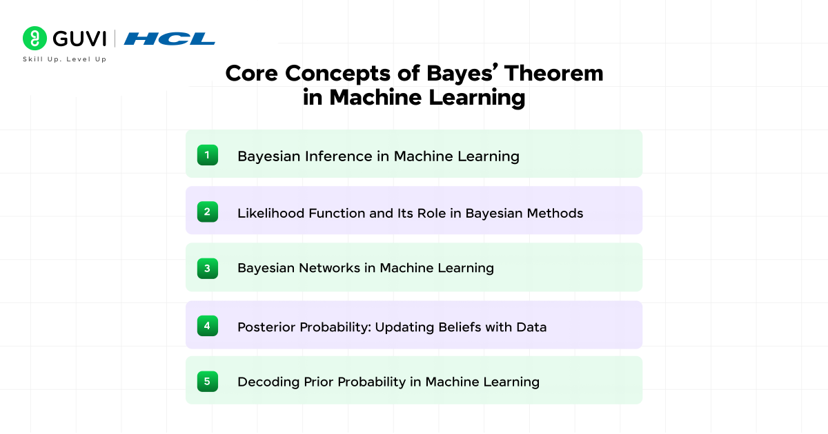
Here are the leading concepts of Bayes’ Theorem in Machine Learning:

1. Bayesian Inference in Machine Learning

What is Bayesian Inference?

Bayesian inference is the process of updating probability estimates as new data arrives. It treats model parameters as random variables and uses Bayes’ Theorem to move from a prior distribution to a posterior distribution. The posterior then becomes the new prior when additional evidence is gathered.

Bayesian Inference Machine Learning Applications

In practice, Bayesian inference appears in:

• Naive Bayes classifiers, where class probabilities updated with each feature.
• Bayesian networks capture dependencies among multiple variables.
• Hierarchical models, where parameters at one level inform priors at a higher level.
• Gaussian processes, for regression and function approximation with uncertainty estimates.

How to Update Beliefs with New Data?

Updating beliefs follows a simple cycle:

1. Start with a prior distribution over model parameters.
2. Observe new data and compute the likelihood of that data under each parameter setting.
3. Multiply the prior by the likelihood and normalize to obtain the posterior distribution.
4. Use the posterior as the prior for the next round of data.

This iterative loop ensures that a model remains current. Each pass through data refines parameter estimates and improves predictive performance under uncertainty.

Also Read: Logistic Regression in Machine Learning: A Complete Guide

2. Likelihood Function and Its Role in Bayesian Methods

What is a Likelihood Function?

A likelihood function assigns a score to each possible set of parameter values. This assignment is based on how probable the observed data would be if those values were true. It is not a probability distribution over parameters but rather a function of parameters given data.

Role of Likelihood in Updating Posterior Probabilities

In Bayesian methods, the likelihood determines the weight that new data places on different parameter values. When you multiply the prior by the likelihood, high-likelihood regions of the prior get boosted in the posterior. Low-likelihood regions shrink. The result is a posterior distribution that balances prior assumptions with actual observations.

3. Bayesian Networks in Machine Learning

What are Bayesian Networks?

A Bayesian network is a graph that encodes probabilistic relationships among a set of variables. Nodes represent random variables, and edges represent direct dependencies. Each node carries a conditional probability table that defines how it relates to its parents in the graph.

How Bayesian Networks Model Probabilistic Relationships?

The network structure breaks a complex joint distribution into a product of simpler conditional distributions. If variable A depends on B and C, then P(A, B, C) equals P(A | B, C) times P(B) times P(C), and so on for all variables. That factorization reduces computation and clarifies which variables directly influence others.

Practical Examples of Bayesian Networks

Bayesian networks appear in medical diagnosis, where symptoms and diseases form a dependency graph. They also power fault detection systems in engineering, where component failures propagate through a network. In each case, the network lets you update probabilities across all variables when you observe new evidence.

4. Posterior Probability: Updating Beliefs with Data

Posterior probability is expressed as P(H|D), and it represents the updated belief about the hypothesis after taking into account the observed data. Calculating the posterior involves combining the prior probability with the likelihood and then normalizing by the probability of the data across all possible hypotheses. 

This process implements the idea of learning from data. The posterior serves as the updated probability distribution that reflects both historical knowledge and new evidence. The posterior from one update becomes the prior for the next in iterative settings. It further allows continuous adaptation as additional data becomes available.

The Conditional Probability Formula in Bayesian Learning

Conditional probability in Bayes’ Theorem in machine learning remains fundamental throughout the Bayesian learning framework. The conditional probability formula formalizes the relationship between:

• Prior probability
• Likelihood
• Posterior probability

This structure enables systematic probability updates as data accumulates. Conditional probability shows up directly in the way we approach problems like classifying images or grouping similar data points. Even when a model tries to express how confident it is in its predictions, conditional probability is at the root of that process.

5. Decoding Prior Probability in Machine Learning

What is Prior Probability?

To apply Bayes’ Theorem in machine learning, a precise definition of the prior probability is essential. The prior probability is commonly represented as P(H). It describes the initial belief about a hypothesis before any observation of data. The prior incorporates assumptions, domain expertise, or empirical evidence about the frequency or plausibility of specific outcomes in practical settings.

Types of Priors

• Informative priors: based on strong domain knowledge or historical data (e.g., medical incidence rates).
• Non-informative (or weak) priors: intentionally vague (e.g,. uniform), letting the data “speak for itself.”

Impact on Posterior & Learning

• A strong prior can dominate when data are sparse, stabilizing estimates but risking bias if the prior is mis‐specified.
• A weak prior yields data‐driven posteriors but may lead to overfitting or high variance with limited observations.

Practical Considerations

• Choosing an appropriate prior involves balancing domain expertise with data availability.
• Sensitivity analyses (testing different priors) help gauge how much your results depend on those initial assumptions.

Want to master Bayes’ Theorem and apply probabilistic reasoning to real-world ML projects? Join the Intel & IITM Pravartak certified program, trusted by over 3.5 million learners and partnered with 1000+ top tech employers. 

Gain practical skills that set you apart and a certification that’s recognized across the industry. Register for HCL GUVI AI/ML Course to to open the door to your future in machine learning. Register now and turn foundational theory into measurable career growth!

The Mathematics: Bayes’ Theorem Formula for Machine Learning

The Conditional Probability Formula

For any events AA and BB with P(B)>0P(B)>0, Bayes’ Theorem states:

Here:

• P(A)P(A): the prior probability of hypothesis AA before observing any evidence.
• P(B∣A)P(B∣A): the likelihood: the probability of seeing evidence BB when AA is true.
• P(B)P(B): the marginal (or evidence) probability of BB, given by,

where {Ai}{Ai​} is a partition of all possible hypotheses.

P(A∣B)P(A∣B), the posterior probability of AA after observing BB.

In Machine Learning

• Classification: Let AA be a class label and BB the observed features. We compute:

and predict the label with the highest posterior.

• Parameter estimation: Let AA be a model’s parameters and BB the data. Bayes’ Theorem gives the posterior distribution over parameters, quantifying uncertainty in those estimates.

Simple Bayes’ Theorem Example in Machine Learning

Consider a spam-detection model.

Suppose:

• 20% of emails are spam.
• 70% of spam emails contain the word “offer”.
• 10% of legitimate emails contain the word “offer”.

We want to calculate the probability that an email is spam after observing the word “offer”.

The prior is:

P(Spam) = 0.20

The likelihood is:

P(Offer|Spam) = 0.70

The probability of observing “offer” is:

P(Offer) = (0.70 × 0.20) + (0.10 × 0.80)

P(Offer) = 0.22

Now apply Bayes’ Theorem:

P(Spam|Offer) = (0.70 × 0.20) / 0.22

P(Spam|Offer) ≈ 0.636

The probability that the email is spam rises from 20% to about 63.6% after the new evidence appears.

This simple example shows why Bayes’ Theorem is useful. The model does not discard its earlier knowledge. It combines prior information with new evidence.

Advantages and Limitations of Bayesian Methods

Key Advantages

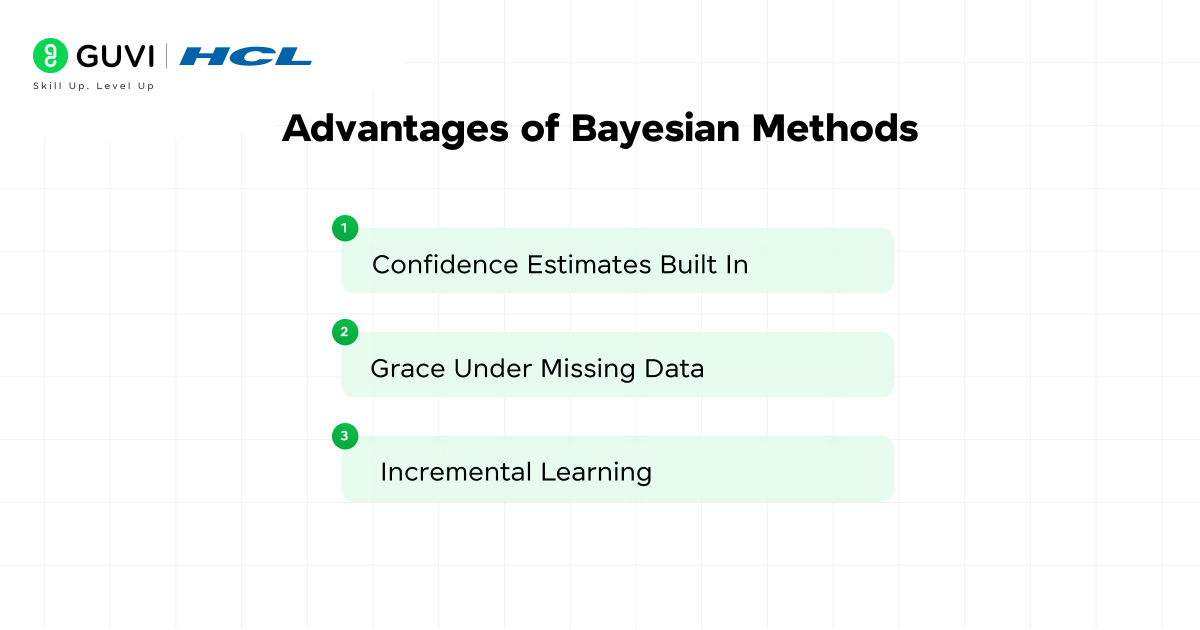
• Confidence estimates built in. Every prediction returns a probability distribution instead of a single point. You see whether the model is barely sure or almost certain, and that insight guides decisions when stakes are high.
• Grace under missing data. When some features go missing, a well-chosen prior can fill the gaps. The model keeps working, and you avoid the crash-and-retrain cycle.
• Incremental learning. Once you compute a posterior, you plug it back in as the next prior. The model evolves as data arrive, never throwing away past learning or demanding full retraining.

Common Limitations and How to Address Them

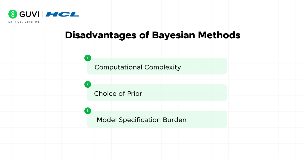
• Computational complexity. Exact posterior calculation in high dimensions often needs integrals you cannot solve by hand. Switch to variational inference or expectation propagation. They trade a bit of accuracy for tractability and let you scale to real-world problems.
• Choice of prior. The wrong prior can bias results. Test multiple priors and compare posteriors. If they converge on similar parameter ranges, your inferences are robust. Use weakly informative priors to set sensible bounds without overcommitting.
• Model specification burden. Designing complex hierarchical models or full Bayesian networks can become overwhelming. Start with a simple structure and validate it on held-out data. Then, add layers only as the use case demands. That stepwise approach keeps inference problems manageable and helps you catch specification errors early.

Practical Applications and Case Studies

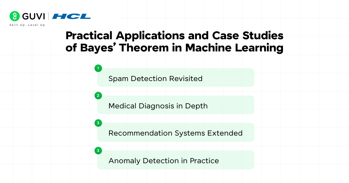
Below are detailed examples of projects that put Bayes’ Theorem to work in real settings:

1. Spam Detection Revisited

Email filters based on Naive Bayes remain a staple. They start with priors on word frequencies for spam versus legitimate mail and update those priors as each new message arrives. This makes it simple to incorporate new vocabulary without rebuilding the entire model.

Key steps in the data flow:

1. Count word occurrences separately in spam and non-spam datasets.
2. Compute the likelihoods P(word | spam) and P(word | non-spam) from those counts.
3. Multiply each likelihood by the prior spam rate P(spam).
4. Normalize over both classes to obtain the posterior P(spam | message).

Monthly re-estimation of word counts keeps the classifier in sync with evolving spam tactics and emerging keywords.

2. Medical Diagnosis in Depth

Bayesian networks link diseases, symptoms and test results through directed edges and conditional probability tables. When a new lab result comes in, the network recalculates posteriors across all related nodes, giving clinicians updated probabilities for each condition and symptom.

Setup for a simple diagnostic network:

• Nodes representing Disease, Symptom A, Symptom B, and Test Result
• Directed links flowing from Disease to each Symptom and to Test Result

Update cycle:

1. Enter the patient’s Test Result (positive or negative) into the network.
2. Update the posterior P(Disease | Test).
3. Propagate changes to symptom nodes, revising P(Symptom | Disease, Test).
4. Present final posteriors for both disease probabilities and symptom likelihoods to the clinician.

This process guides decisions on follow-up tests and helps prioritize treatment options based on quantified risk.

3. Recommendation Systems Extended

In content and product recommendations, a user’s initial preferences serve as the prior. Each click or purchase acts as new evidence, updating item-specific scores in real time or in batches.

Batch update procedure:

1. After accumulating a set number of interactions (for example, 100), recompute posteriors for each user–item pair.
2. Model click/no-click outcomes with a Beta-Bernoulli framework, where the Beta prior captures past behavior and the Bernoulli likelihood represents recent interactions.

Real-time update strategy:

• Apply a streaming update rule that adjusts posteriors immediately after each event.
• Give greater weight to recent clicks by tuning the likelihood function, ensuring the system adapts quickly to changing user interests.

4. Anomaly Detection in Practice

Monitoring systems for servers or sensor networks establish a baseline distribution of “normal” readings using Bayesian estimates. Readings that fall into the low-probability tails trigger alerts, which further allow rapid response to potential faults.

Model choices:

• Use a Gaussian model for continuous metrics such as CPU load or temperature.
• Apply a Dirichlet-multinomial model for categorical counts like error codes or event types.

Thresholding approach:

1. Define an alert threshold, for example, P(normal | reading) < 0.01.
2. Calibrate the threshold based on acceptable false-alarm rates and operational risk tolerance.

This setup ensures that genuine anomalies stand out reliably while minimizing unnecessary alerts.

Best Practices for Implementing Bayesian Approaches

1. Select realistic priors, informed by domain expertise or weakly informative distributions.
2. Choose scalable inference methods such as MCMC, variational inference or Laplace approximation, matching them to model size and performance requirements.
3. Validate model assumptions through posterior predictive checks, comparing simulated data against real observations.
4. Monitor convergence diagnostics, effective sample size and potential scale reduction factor to ensure reliable posterior estimates.
5. Test sensitivity to prior choices by running analyses with alternative priors and comparing results.
6. Calibrate probability estimates using methods like isotonic regression or Platt scaling so predicted confidences match observed frequencies.
7. Automate incremental updates by feeding each posterior back in as the next prior, avoiding full retraining when new data arrives.
8. Apply model selection criteria: Bayes factors, WAIC or cross-validation to compare competing Bayesian formulations.
9. Document prior specifications, likelihood definitions and update procedures for reproducibility.
10. Perform out-of-sample validation on held-out data to assess predictive accuracy under real-world conditions.

Complete Guide to Learning Bayes’ Theorem in Machine Learning in India 2026

For learners in India, Bayes’ Theorem is best studied as part of a broader machine learning foundation instead of as an isolated probability formula.

A practical 2026 learning path can follow this sequence:

Step 1: Build Probability Fundamentals

Start with:

• Conditional probability
• Random variables
• Probability distributions
• Expected value
• Variance
• Joint and marginal probability

These concepts make Bayes’ Theorem considerably easier to understand.

Step 2: Learn the Bayes Formula

Understand each part of the equation:

• Prior
• Likelihood
• Evidence
• Posterior

Then solve simple examples manually before writing code.

Step 3: Implement Naive Bayes

Build small classification projects using:

• Gaussian Naive Bayes
• Multinomial Naive Bayes
• Bernoulli Naive Bayes

Text classification is an effective starting point.

Step 4: Move Into Bayesian Inference

Once the basic theorem is clear, study:

• Posterior distributions
• Prior selection
• MCMC
• Variational inference
• Posterior predictive checking

Step 5: Build Portfolio Projects

Useful beginner and intermediate projects include:

• Spam email classification
• Sentiment classification
• Disease-risk estimation
• Customer conversion modelling
• Bayesian A/B testing
• Recommendation modelling
• Bayesian network-based fault detection

Step 6: Learn the 2026 Bayesian ML Tool Stack

The current Python ecosystem provides several mature tools for Bayesian machine learning.

Python 3.14.6 was released in June 2026. scikit-learn lists 1.9.0 as its stable release. PyMC 6.3.1 was released on Aug. 16, 2026. pgmpy 1.1.2 is its latest published release. CmdStan 2.39.0 arrived in 2026 and ArviZ 1.3.0 was released in August 2026.

The right tool depends on the problem. scikit-learn is suitable for learning Naive Bayes classification. PyMC and Stan are better suited to custom probabilistic models. pgmpy focuses on graphical models while ArviZ supports Bayesian model analysis.

The Bottom Line

Bayes’ Theorem gives machine learning systems a structured way to learn from evidence under uncertainty. The process begins with a prior belief. New observations contribute likelihood information. Both are combined to calculate a posterior probability.

This simple idea supports methods ranging from Naive Bayes classification to Bayesian networks, probabilistic programming and Bayesian optimization. Learning the theorem is therefore more than memorizing a formula. Understanding priors, likelihoods, posterior distributions and uncertainty gives you a stronger foundation for modern machine learning.

FAQs