Backpropagation Algorithm in Machine Learning

Every time a neural network learns to recognise a cat, translate a sentence, or predict tomorrow’s stock price, one algorithm is responsible for making that learning happen: backpropagation.

Backpropagation, short for backward propagation of errors, is the training algorithm that makes deep learning possible. It calculates how much each weight in a neural network contributed to the prediction error, and uses that information to adjust every weight in a direction that reduces future errors. Without it, training a network with more than one hidden layer would be computationally intractable.

Despite its centrality to modern AI, backpropagation is often presented as a black box — something that “just works” inside frameworks like TensorFlow and PyTorch. This article pulls back the curtain: explaining what backpropagation is, how it works mathematically and intuitively, and why it remains the cornerstone of deep learning after more than three decades.

TL;DR

• Backpropagation computes gradients of the loss function with respect to every weight in the network using the chain rule.
• It operates in two passes: a forward pass that produces predictions, and a backward pass that propagates error signals.
• The computed gradients are used by gradient descent to update weights in the direction that reduces the loss.
• Activation functions must be differentiable for backpropagation to work;k this is why choices like ReLU and sigmoid matter.
• Backpropagation is the foundational training algorithm for virtually all modern deep learning architectures.

The Problem Backpropagation Solves

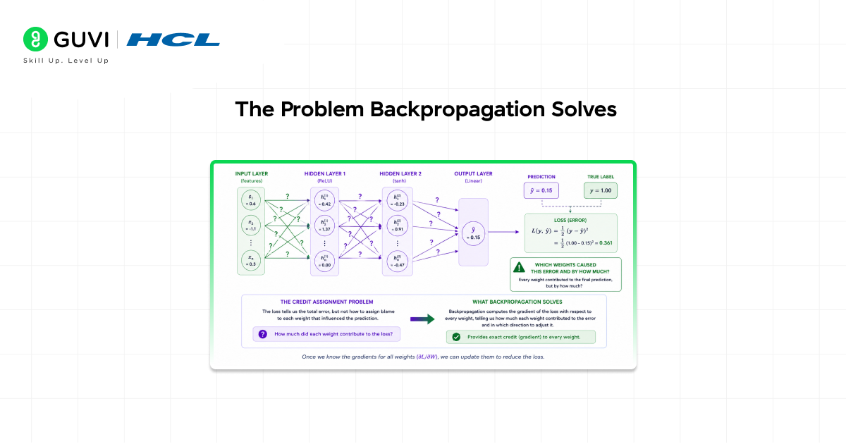
To understand why backpropagation matters, it helps to understand the problem it was designed to solve: the credit assignment problem.m 

The Credit Assignment Problem

A neural network with multiple layers contains thousands, sometimes billions of weights. When the network makes a wrong prediction, the error is visible at the output layer. But which weights were responsible? And by how much should each one be adjusted?

In a shallow network with no hidden layers, the answer is straightforward: the output weights are directly connected to the prediction. But in a deep network with many hidden layers, the relationship between any individual weight and the final error is indirect, mediated by every layer between that weight and the output.

This is the credit assignment problem: efficiently determining the contribution of each weight to the overall prediction error, across many layers and many thousands of parameters.

Why Early Approaches Failed

Before backpropagation, training multi-layer networks required either finite difference approximations, estimating gradients by perturbing each weight individually, which requires a full forward pass per weight and scales disastrously or random weight perturbation methods that were too slow and imprecise to be practical.

Backpropagation solved this by applying the chain rule of calculus to compute exact gradients for every weight in a single backward pass. What would take thousands of forward passes to approximate with finite differences, backpropagation computes exactly in two passes, one forward, one backward.

Forward Pass: From Input to Prediction

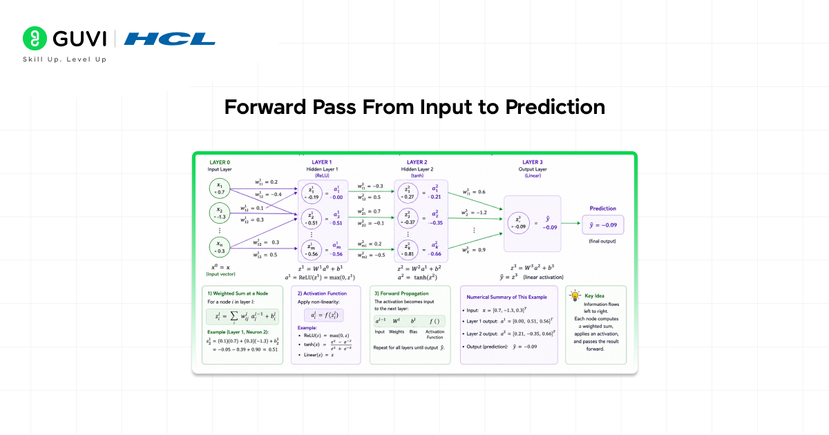
Backpropagation consists of two phases. The first is the forward pass, which produces the network’s prediction. Understanding the forward pass precisely is essential before the backward pass makes sense.

Layer-by-Layer Computation

In the forward pass, data flows from the input layer through each hidden layer to the output layer. At each neuron in each layer, two operations occur:

1.  Weighted sum: The neuron computes the weighted sum of its inputs, each input multiplied by its corresponding connection weight, plus a bias term. This is the pre-activation value, often called z.

2.    Activation function: The activation function is applied to z, producing the neuron’s output, its activation value a. This output becomes the input to every neuron in the next layer.

The activation function is critical. It introduces non-linearity into the network, enabling it to learn complex, non-linear patterns. Without activation functions, a deep network would reduce to a single linear transformation regardless of depth. Common activation functions include:

• Sigmoid: Squashes inputs to the range (0, 1). Historically popular for output layers in binary classification. Prone to vanishing gradients in deep networks.
• Tanh: Squashes inputs to the range (-1, 1). Zero-centred, which often leads to faster convergence than sigmoid. Still suffers from vanishing gradients.
• ReLU (Rectified Linear Unit): Returns max(0, z). Computationally efficient and largely mitigates the vanishing gradient problem. The default choice for hidden layers in modern deep networks.
• Softmax: Converts a vector of values into a probability distribution that sums to 1. Used in output layers for multi-class classification problems.

Computing the Loss

After the forward pass produces a prediction, the loss function measures how far that prediction is from the correct answer. The choice of loss function depends on the task:

• Mean Squared Error (MSE): Used for regression tasks. Measures the average squared difference between predictions and true values.
• Binary Cross-Entropy: Used for binary classification. Measures the divergence between predicted probabilities and true binary labels.
• Categorical Cross-Entropy: Used for multi-class classification. Measures the divergence between the predicted class probability distribution and the true one-hot encoded label.

The loss value is a single scalar,r, a summary of how wrong the network’s prediction was. The backward pass will use this value to compute gradients.

Backward Pass: Propagating the Error

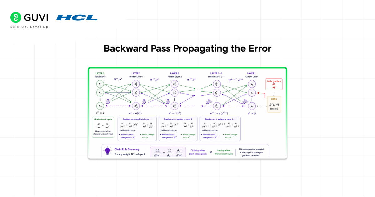
The backward pass is where backpropagation earns its name. It propagates the error signal from the output layer back through the network, computing the gradient of the loss with respect to every weight in the network.

The Chain Rule: The Mathematical Foundation

The chain rule of calculus states that the derivative of a composite function can be computed as the product of the derivatives of its components. Formally, if y = f(g(x)), then:

dy/dx = (dy/dg) × (dg/dx)

A neural network is a deeply nested composite function. The output of the final layer is a function of the outputs of the penultimate layer, which are functions of the outputs of the layer before that, all the way back to the input. The chain rule allows the gradient of the loss with respect to any weight, no matter how many layers deep, to be expressed as a product of local gradients computed at each layer.

This is the mathematical insight that makes backpropagation efficient: instead of computing each gradient independently, the algorithm reuses intermediate values computed during the forward pass, sharing computation across all gradients through a single backward sweep.

Computing Gradients Layer by Layer

The backward pass begins at the output layer. The gradient of the loss with respect to the output layer’s pre-activation values is computed directly from the loss function and the activation function’s derivative.

This gradient is then propagated backward to the previous layer. For each layer, the backward pass computes:

•    Gradient with respect to weights: How much does the loss change if this weight changes slightly? This is the value used to update the weight.

•   Gradient with respect to biases: How much does the loss change if this bias changes slightly? Used to update the bias term.

•     Gradient with respect to layer inputs: How much does the loss change if this layer’s input changes slightly? This becomes the gradient passed to the previous layer, continuing the backward propagation.

This process repeats for every layer from output back to input, accumulating the gradient signal and distributing it to every weight in the network.

Weight Update: From Gradients to Learning 

Computing gradients is the core of backpropagation, but gradients alone do not change the network. The weight update step implemented by gradient descent applies the gradients to modify every weight in the direction that reduces the loss.

The Gradient Descent Update Rule

The fundamental weight update rule is:

w ← w − η × (∂L / ∂w)

Where:

•        w: The current weight value.

•        η (eta): The learning rate is a hyperparameter that controls how large each update step is.

•        ∂L / ∂w: The gradient of the loss function with respect to this weight, computed by backpropagation.

The negative sign is critical: subtracting the gradient moves the weight in the direction of steepest descent on the loss surface toward a minimum. Gradients point toward the steepest increase in loss; moving against the gradient reduces it.

The Learning Rate: A Critical Hyperparameter

The learning rate determines how aggressively the network updates its weights at each step:

• Too high: Updates overshoot the minimum. The loss oscillates or diverges instead of converging.
• Too low: Training is extremely slow. The network makes minimal progress per update and may get stuck in local minima or plateau regions.
• Well-tuned: The network converges efficiently toward a good solution without oscillation or stagnation.

Modern practice uses adaptive learning rate methods, such as Adam, RMSProp, and AdaGrad, that automatically adjust the effective learning rate for each weight based on the history of its gradients, significantly reducing the sensitivity to learning rate choice.

Mini-Batch Gradient Descent

In practice, weight updates are not computed using a single training example (stochastic gradient descent) or the entire dataset (batch gradient descent) — they use mini-batches: small random subsets of the training data, typically 32 to 256 examples. This approach:

•        Provides gradient estimates that are more stable than single-example updates.

•        Fits naturally into GPU parallelism, which processes batches simultaneously.

•        Introduces beneficial noise that helps the network escape sharp local minima.

The Vanishing and Exploding Gradient Problems

Backpropagation has two well-known failure modes that become more severe as network depth increases: vanishing gradients and exploding gradients. Both arise from the multiplicative nature of the chain rule.

Vanishing Gradients

During the backward pass, the chain rule multiplies local gradients together across every layer. If these local gradients are consistently less than 1, as they are for the sigmoid and tanh activation functions in their saturated regions, the product of many such values becomes exponentially small.

The result is that gradients flowing back to the early layers of the network become vanishingly small. Early layers update their weights by an imperceptible amount, effectively failing to learn. This is why deep networks trained with sigmoid activations often fail to learn good representations in their early layers.

Solutions include:

• ReLU activations: Have a gradient of exactly 1 for positive inputs, preventing the compounding shrinkage.
• Batch Normalisation: Normalises layer outputs to keep activations in a range where gradients remain healthy.
• Residual connections (skip connections): Allow gradients to flow directly to earlier layers without passing through every intermediate layer, the key innovation of ResNet architectures.

Exploding Gradients

The opposite problem occurs when local gradients are consistently greater than 1. The chain rule product grows exponentially with depth, producing gradient values so large that weight updates become unstable, and the network diverges rather than converges.

Solutions include:

• Gradient clipping: Caps the gradient magnitude at a defined threshold before the update step, preventing individual updates from being catastrophically large.
• Careful weight initialisation: Schemes like Xavier/Glorot and He initialisation set initial weight values to keep gradient magnitudes in a stable range from the start of training.

Backpropagation Through Time (BPTT) 

Standard backpropagation operates on feedforward networks where information flows in one direction from input to output. Recurrent neural networks (RNNs), however, have connections that loop back on themselves, allowing information to persist across sequential inputs. Training RNNs requires a variant of backpropagation called Backpropagation Through Time (BPTT).

How BPTT Works

BPTT unrolls the recurrent network across time steps, treating the RNN as a very deep feedforward network where each “layer” corresponds to one time step. Standard backpropagation is then applied through this unrolled network, computing gradients with respect to the shared weights at each time step and summing them.

The challenge of BPTT is that RNNs applied to long sequences produce very deep unrolled networks, making them particularly susceptible to the vanishing and exploding gradient problems. This is why Long Short-Term Memory (LSTM) and Gated Recurrent Unit (GRU) architectures were developed. They use gating mechanisms that allow gradients to flow across long sequences without vanishing.

Backpropagation in Modern Deep Learning

Backpropagation is not just a training algorithm for simple networks; it scales to the largest AI systems ever built. Every major architecture in modern deep learning relies on backpropagation for training.

• Convolutional Neural Networks (CNNs): Backpropagation computes gradients through convolutional layers, pooling layers, and fully connected layers to train image classification, object detection, and image generation models.
• Recurrent Neural Networks and LSTMs: BPTT trains sequence models for language modelling, speech recognition, and time-series prediction.
• Transformers and Large Language Models: The attention mechanism in transformer architectures is fully differentiable, allowing backpropagation to train models with hundreds of billions of parameters across distributed GPU clusters. GPT-4, Claude, and Gemini are all trained using backpropagation.
• Generative Adversarial Networks (GANs): Backpropagation trains both the generator and discriminator in the adversarial training loop.
• Variational Autoencoders (VAEs): Backpropagation flows through the encoder, the reparameterisation trick, and the decoder to optimise the evidence lower bound.

Modern deep learning frameworks TensorFlow, PyTorch, and JAX implement automatic differentiation (autograd) systems that automatically compute and apply backpropagation gradients for any network architecture defined by the user. This automation is what has made the explosive growth of deep learning research and deployment possible.

If you want practical experience working with activation functions, neural networks, and deep learning models, HCL GUVI’s AI and ML Course can help you understand how concepts like sigmoid, backpropagation, and gradient descent are implemented using frameworks such as TensorFlow and PyTorch through hands-on projects. 

Conclusion

The backpropagation algorithm is the engine of deep learning. By applying the chain rule of calculus in a single efficient backward pass through a neural network, it solves the credit assignment problem, determining exactly how each weight contributed to the prediction error and how it should be adjusted to reduce future errors.

From its mathematical roots in the chain rule to its practical implementation in automatic differentiation frameworks, backpropagation has proven remarkably robust. It trains convolutional networks on images, recurrent networks on sequences, transformers on language, and networks with hundreds of billions of parameters that power the most capable AI systems in existence today.

Understanding backpropagation is not just an academic exercise. It is foundational knowledge that explains why certain architectures work, and others fail, why activation function choice matters, why gradient flow must be managed carefully in deep networks, and how the learning dynamics of neural networks can be debugged and improved. For anyone serious about machine learning, backpropagation is where deep understanding begins.

FAQs

1. What is backpropagation in simple terms?

Backpropagation is the algorithm that teaches neural networks by calculating how much each weight contributed to the prediction error and adjusting every weight to reduce that error. It works by applying the chain rule of calculus in a backward pass from the output to the input layer.

2. What is the difference between backpropagation and gradient descent?

Backpropagation computes the gradients; it tells you how much each weight should change. Gradient descent uses those gradients to actually update the weights. Backpropagation and gradient descent always work together: backpropagation provides the gradients, gradient descent applies them.

3. Why do activation functions need to be differentiable?

Backpropagation applies the chain rule through the activation function at each layer. This requires computing the derivative of the activation function. Non-differentiable functions block gradient flow and make backpropagation impossible,e which is why ReLU, despite having a non-differentiable point at zero, uses a subgradient convention in practice.

4. What causes the vanishing gradient problem?

Vanishing gradients occur when local gradients, particularly the derivatives of sigmoid and tanh activation functions,  are less than 1. Multiplying many such values together during the backward pass produces exponentially small gradients in early layers, which effectively stop learning. ReLU activations and residual connections are the primary solutions.

5. Is backpropagation used in all deep learning models?

Yes. Backpropagation implemented through automatic differentiation frameworks trains virtually all modern deep learning architectures, including CNNs, RNNs, transformers, GANs, and VAEs. Any architecture defined as a composition of differentiable operations can be trained with backpropagation.