


Artificial Intelligence and Machine Learning Articles
How to Evaluate LLM Outputs in Production Deployments
AI/ML Skills Gap 2026: Why Companies Can't Find Job-Ready Talent
20 AI/ML Interview Questions Recruiters Can Use Without a Tech Background - Best Guide
How Industry-Backed AI/ML Bootcamps Are Changing the AI/ML Hiring Pipeline - Best Guide 2026


Get In Touch For Details! Request More Information

A* Algorithm in AI: Finding the Optimal Path Fast
Sep 25, 2026 11 Min Read 1456 Views
(Last Updated)
Finding a path between two points is easy when the search space is small. The challenge begins when an AI system must choose the lowest-cost route across thousands or millions of possible states without exploring every option.
The A algorithm in AI* solves this problem by combining the actual cost already travelled with a heuristic estimate of the remaining cost. This allows A* to prioritize promising paths while still finding an optimal solution when the heuristic satisfies the required conditions.
A* is widely studied in artificial intelligence because its core ideas apply beyond map navigation. The same search strategy can support game pathfinding, robotics, automated planning, puzzle solving, and other problems that can be represented as weighted graphs.
This guide explains how the A* algorithm works, its f(n) = g(n) + h(n) formula, heuristic functions, Python implementation, real-world applications, complexity, optimization techniques, and how it compares with other pathfinding algorithms.
Quick Answer
The A algorithm* is an informed search algorithm that finds a lowest-cost path by combining the cost already travelled with an estimate of the remaining cost.
- Core Formula:
f(n) = g(n) + h(n). - g(n): Actual path cost from the start node to the current node.
- h(n): Heuristic estimate from the current node to the goal.
- Node Selection: A* expands the node with the lowest estimated total cost
f(n). - Optimality: A* can return an optimal solution when its heuristic satisfies the necessary admissibility and consistency conditions.
Table of contents
- The Problem A* Solves: Pathfinding in a Graph
- The Problem A Solves: Pathfinding in a Graph*
- The A* Formula: f(n) = g(n) + h(n)
- How A* Works: Step-by-Step
- A* Algorithm: Python Implementation
- Admissible vs Consistent Heuristics in the A Algorithm*
- What Is an Admissible Heuristic?
- What Is a Consistent Heuristic?
- Admissible vs Consistent
- A vs Dijkstra vs Greedy Best-First Search*
- Dijkstra's Algorithm
- Greedy Best-First Search
- A*
- Time and Space Complexity of the A Algorithm*
- Time Complexity
- Space Complexity
- How Heuristic Quality Affects Performance
- Common A Algorithm Mistakes and Optimization Techniques*
- Using an Incorrect Heuristic
- Not Updating a Node When a Cheaper Path Is Found
- Using an Inefficient Open List
- Storing Complete Paths for Every Queue Entry
- Ignoring Duplicate Queue Entries
- Using Standard A on Extremely Large Search Spaces*
- Real-World Applications of A* in Artificial Intelligence
- Navigation and Mapping
- Video Game AI and Pathfinding
- Robotics and Motion Planning
- Network Routing
- AI Planning and Problem Solving
- Can the A Algorithm Work on Directed Graphs?*
- How Does State Representation Affect A Performance?*
- How Does A Handle Multiple Goal States?*
- Can A Search Continuous State Spaces?*
- How Does A Handle Changing Maps or Edge Costs?*
- Conclusion
- FAQs
- Is A* always guaranteed to find the optimal path?
- What is the difference between an admissible and a consistent heuristic?
- What is the time complexity of A*?
- How is A* different from Dijkstra's algorithm?
- Can A* handle dynamic environments where edges or costs change?
- What is the difference between an AI course and an AI & ML course?
- Why is SQL important for AI & ML professionals?
- What job roles can I apply for after completing an AI & ML course?
- How do I choose the best AI course for my career goals?
- What should I look for before enrolling in an AI & ML course?
- How should I evaluate AI & ML certifications before enrolling?
What Is the A* Algorithm?
The A* (A-star) algorithm is an informed heuristic search algorithm used in artificial intelligence to find the shortest or least-cost path between a start node and a goal node in a weighted graph. It evaluates nodes using the function f(n) = g(n) + h(n), where g(n) represents the known cost from the start node to the current node and h(n) is a heuristic estimate of the remaining cost to the goal. When the heuristic is admissible, meaning it never overestimates the true cost, A* is guaranteed to find the optimal path.
The Problem A* Solves: Pathfinding in a Graph
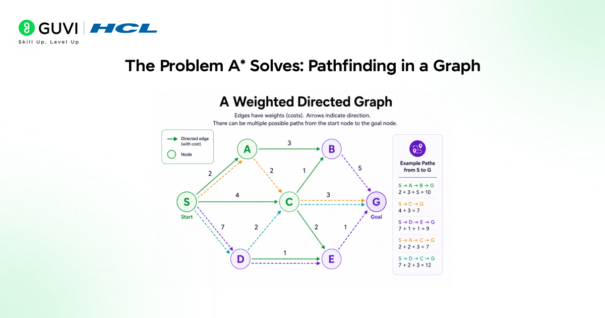
The Problem A Solves: Pathfinding in a Graph*
Before understanding A*, it is important to understand the problem it solves: finding the lowest-cost path between two states in a weighted graph.
In AI, a graph represents a problem as:
- Nodes: Possible states or locations.
- Edges: Valid transitions between those states.
- Edge Costs: The cost of moving from one node to another, such as distance, time, fuel, risk, or energy.
- Start Node: The state where the search begins.
- Goal Node: The destination the algorithm must reach.
For example, in a navigation system, cities or intersections become nodes, roads become edges, and travel time or distance becomes the edge cost. In a game, map positions become nodes while valid movements between positions become edges.
The pathfinding problem is therefore:
Find a sequence of connected nodes from the start to the goal whose total edge cost is minimum.
Suppose there are two possible routes:
- Route A: Start → B → Goal = 18 units
- Route B: Start → C → D → Goal = 12 units
A correct shortest-path algorithm should choose Route B, even though it contains more intermediate nodes, because its total path cost is lower.
Uninformed search algorithms such as Breadth-First Search and Depth-First Search do not use an estimate of how close a state is to the goal.
BFS explores nodes level by level and can find a shortest path when all edges have equal cost. DFS explores one branch deeply before backtracking and does not guarantee the lowest-cost path.
A* improves this search by combining two values:
Actual cost already travelled + Estimated cost remaining to the goal
This heuristic guidance allows A* to prioritize nodes that appear more promising instead of exploring the search space uniformly. As a result, it can reach an optimal path while examining far fewer irrelevant states when the heuristic is well designed.
The A* Formula: f(n) = g(n) + h(n)
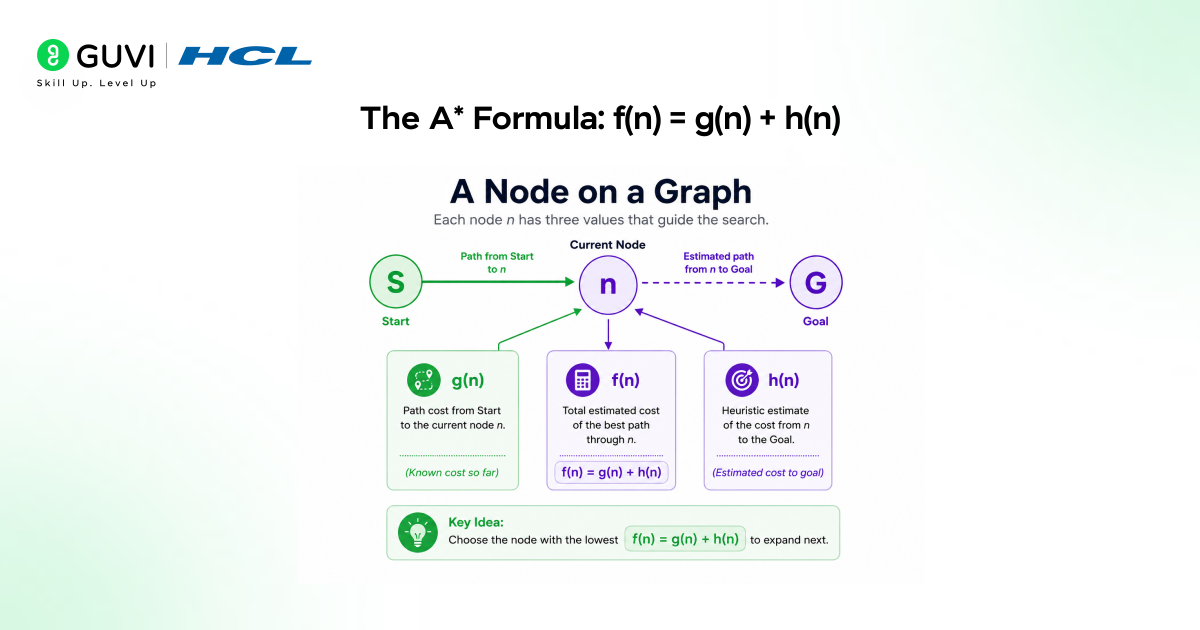
The A* algorithm evaluates every candidate node using a score that estimates the total cost of reaching the goal through that node:
f(n) = g(n) + h(n)
Each part of the formula has a specific role:
- g(n): Known Path Cost
g(n)is the exact accumulated cost from the start node to the current node. For example, if Start → A costs 4 and A → B costs 3, theng(B) = 7. If A* later finds a cheaper route to B, it updates the value. - h(n): Heuristic Estimate
h(n)estimates the remaining cost from the current node to the goal. It is not the actual cost. It is calculated using a heuristic suited to the problem. - Manhattan Distance: Best suited to grids where movement is limited to horizontal and vertical directions.
- Euclidean Distance: Measures the straight-line distance between two points and is useful when movement can occur in multiple directions.
- Chebyshev Distance: Useful when horizontal, vertical, and diagonal moves are allowed with equal cost.
- f(n): Estimated Total Cost
f(n)combines the known cost and estimated remaining cost. For example, if Node A hasg(n) = 5andh(n) = 7, thenf(n) = 12. If Node B hasg(n) = 8andh(n) = 2, thenf(n) = 10. - Node Selection: A* chooses the node with the lowest
f(n)value from the open list. In the example above, Node B is explored first because10 < 12. - Why It Works: This combination allows A* to balance the cost already travelled with an estimate of the remaining distance, helping it avoid unnecessary exploration.
The A* algorithm was invented in 1968 by Peter Hart, Nils Nilsson, and Bertram Raphael at the Stanford Research Institute. It was originally developed for the Shakey the Robot project, one of the earliest AI initiatives focused on building a mobile robot capable of perceiving its environment, planning actions, and reasoning about how to reach goals autonomously.
How A* Works: Step-by-Step
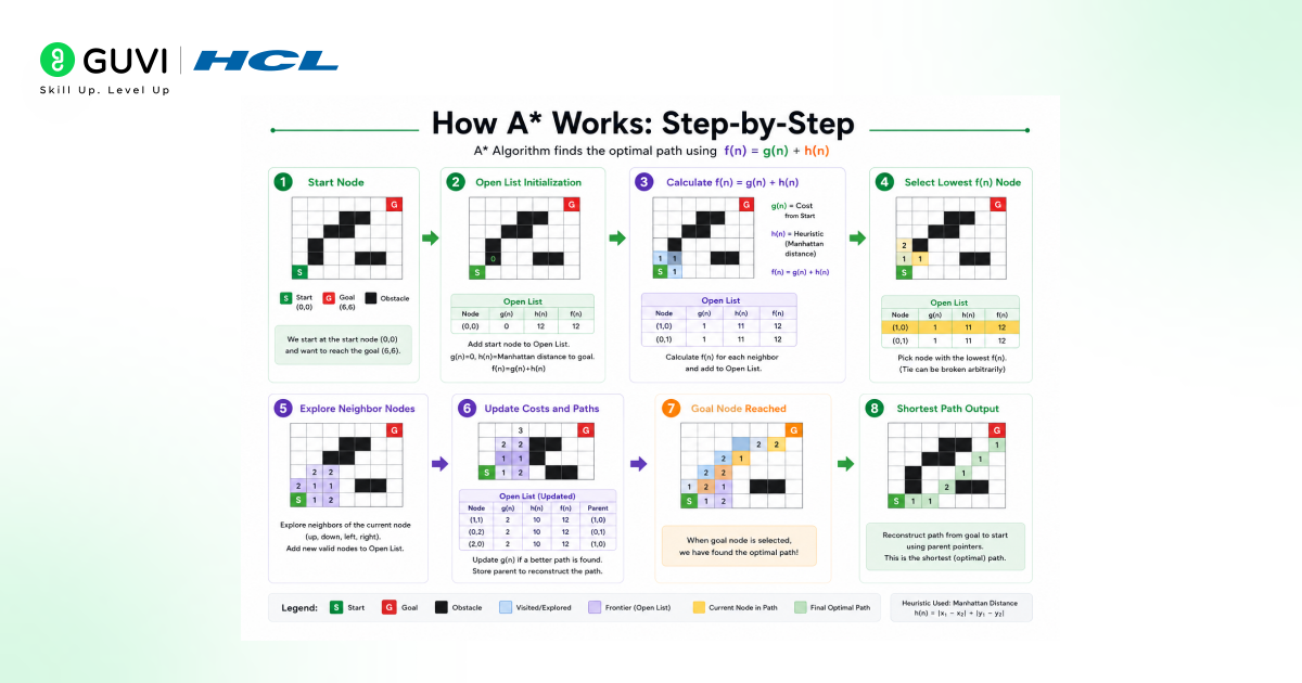
A* maintains two data structures throughout its execution:
- Open list (priority queue): Contains nodes that have been discovered but not yet fully explored. Ordered by f(n) value, the node with the lowest f(n) is always at the front.
- Closed list (visited set): Contains nodes that have already been fully explored. Nodes on the closed list are not re-expanded unless a cheaper path to them is discovered.
The algorithm proceeds as follows: Initialize: Add the start node to the open list with g(start) = 0 and f(start) = h(start).
- Select: Remove the node n with the lowest f(n) value from the open list.
- Goal check: If n is the goal node, the algorithm terminates. Trace back the path using parent pointers to reconstruct the optimal route.
- Expand: For each neighbour n’ of n, calculate the tentative cost: g_tentative = g(n) + cost(n, n’).
- Update: If n’ is not in the open or closed list, or if g_tentative is less than n’s current g(n’) value, update n’s g, f, and parent values, and add n’ to the open list.
- Archive: Add n to the closed list.
- Repeat: Return to step 2. If the open list becomes empty without reaching the goal, no path exists.
The priority queue ensures that A* always expands the most promising node,e the one with the lowest total estimated cost, rather than blindly exploring in all directions.
A* Algorithm: Python Implementation
Here is a clean Python implementation of A* for a weighted graph, illustrating the core logic:
| import heapq def astar(graph, start, goal, heuristic): # open_list: (f(n), g(n), node, path) open_list = [] heapq.heappush(open_list, (heuristic(start, goal), 0, start, [start])) closed_set = set() while open_list: f, g, current, path = heapq.heappop(open_list) if current == goal: return path, g # optimal path and total cost if current in closed_set: continue closed_set.add(current) for neighbour, cost in graph[current].items(): if neighbour not in closed_set: g_new = g + cost f_new = g_new + heuristic(neighbour, goal) heapq.heappush(open_list, (f_new, g_new, neighbour, path + [neighbour])) return None, float(‘inf’) # no path found |
Key implementation notes:
- heapq: Python’s heapq module provides an efficient min-heap, implementing the priority queue with O(log n) insertion and extraction.
- closed_set: A Python set provides O(1) membership checks, ensuring already-expanded nodes are not re-processed.
- Path reconstruction: The path is built incrementally by appending each node to the current path during expansion, avoiding the need for separate parent pointer traversal.
Admissible vs Consistent Heuristics in the A Algorithm*
The performance and correctness of A* depend heavily on the quality of its heuristic function. Two important properties are admissibility and consistency.
What Is an Admissible Heuristic?
A heuristic is admissible when it never estimates a remaining cost higher than the actual minimum cost to reach the goal.
In simple terms:
Estimated remaining cost ≤ True remaining cost
Suppose the actual shortest distance from node A to the destination is 10 km.
These estimates are admissible:
- 6 km
- 8 km
- 10 km
An estimate of 12 km is not admissible because it overestimates the true minimum cost.
An admissible heuristic helps A* preserve optimality under the appropriate graph-search conditions.
What Is a Consistent Heuristic?
A heuristic is consistent when its estimates obey a triangle-like relationship between neighbouring nodes.
For a transition from node n to node n':
h(n) ≤ cost(n, n') + h(n')
This means the estimated cost from the current node should not exceed the cost of moving to a neighbour plus that neighbour’s estimated remaining cost.
Consistency is particularly useful in graph-search implementations because it ensures f(n) values do not decrease along a path.
Admissible vs Consistent
| Property | Admissible Heuristic | Consistent Heuristic |
|---|---|---|
| Main Condition | Never overestimates goal cost | Satisfies the triangle inequality across edges |
| Focus | Accuracy relative to goal | Consistency between neighbouring states |
| Supports Optimal A* | Yes, under appropriate search conditions | Yes |
| Relationship | May not always be consistent | Every consistent heuristic is admissible when h(goal)=0 |
A heuristic that is closer to the true remaining cost while still satisfying the required conditions generally allows A* to explore fewer unnecessary nodes.
A vs Dijkstra vs Greedy Best-First Search*
A* combines ideas from both Dijkstra’s algorithm and Greedy Best-First Search, but the three algorithms prioritize nodes differently.
| Algorithm | Evaluation | Uses Known Cost? | Uses Heuristic? | Main Goal |
|---|---|---|---|---|
| Dijkstra | g(n) | Yes | No | Lowest accumulated path cost |
| Greedy Best-First Search | h(n) | No | Yes | Reach the goal quickly using estimated distance |
| A* | g(n) + h(n) | Yes | Yes | Balance actual and estimated cost |
Dijkstra’s Algorithm
Dijkstra expands the node with the lowest known path cost.
If:
h(n) = 0
for every node, A* behaves like Dijkstra’s algorithm.
Dijkstra does not know which direction the goal lies, so it may explore many nodes that A* can avoid with a useful heuristic.
Greedy Best-First Search
Greedy Best-First Search prioritizes only the heuristic:
f(n) = h(n)
It aggressively moves toward states that appear closest to the goal.
This can make it fast, but ignoring the cost already travelled means it may choose an expensive or suboptimal route.
A*
A* evaluates both:
Actual Cost + Estimated Remaining Cost
This balance is why A* can combine goal-directed search with optimal pathfinding guarantees when the heuristic is appropriately designed.
Time and Space Complexity of the A Algorithm*
The computational cost of A* depends strongly on the graph structure and the quality of the heuristic.
A weak heuristic causes A* to explore more nodes, while an informative heuristic can dramatically reduce the search space.
1. Time Complexity
In difficult search spaces, A* may need to explore an exponential number of nodes.
A commonly discussed worst-case form is:
O(b^d)
where:
b= branching factord= depth of the optimal solution
If each state creates four possible next states and the solution occurs many levels deep, the number of possible nodes can grow rapidly.
However, practical performance can be much better when the heuristic accurately guides the search toward the goal.
2. Space Complexity
Memory is often one of A*’s biggest limitations.
The algorithm may need to store:
- Nodes waiting in the open list
- Previously explored nodes
g(n)valuesf(n)values- Parent information for path reconstruction
As a result, A* can consume substantial memory on extremely large maps or state spaces.
How Heuristic Quality Affects Performance
Consider three cases:
h(n) = 0
A* receives no goal-direction information and behaves like Dijkstra.
Weak but admissible h(n)
A* receives some guidance but may still expand many unnecessary nodes.
Accurate admissible h(n)
A* concentrates more strongly on promising paths and can significantly reduce node expansion.
The best heuristic therefore balances computational simplicity, accuracy, and correctness requirements.
Common A Algorithm Mistakes and Optimization Techniques*
A* is conceptually simple, but implementation details can significantly affect correctness, speed, and memory usage.
1. Using an Incorrect Heuristic
The heuristic must match the movement rules and cost model.
For example:
- 4-direction grid: Manhattan distance is often suitable when horizontal and vertical movement costs are uniform.
- Straight-line movement: Euclidean distance can be appropriate when movement cost corresponds to physical distance.
- 8-direction grid: The appropriate heuristic depends on the relative cost assigned to diagonal and straight movements.
Using an unsuitable heuristic can reduce efficiency and may affect optimality if it overestimates costs.
2. Not Updating a Node When a Cheaper Path Is Found
Suppose A* previously reached node B with:
g(B) = 12
Later, another route reaches B with:
g(B) = 8
The implementation must update B’s cost and parent information when the new route is better.
Ignoring the cheaper path can produce incorrect results.
3. Using an Inefficient Open List
A* repeatedly needs the node with the smallest f(n) value.
A linear search through every open node can become expensive.
A min-priority queue or binary heap allows efficient access to high-priority nodes. Python’s heapq module is commonly used for this purpose.
4. Storing Complete Paths for Every Queue Entry
A simple implementation may attach a complete path to every node placed in the priority queue.
This is easy to understand but can consume unnecessary memory.
For larger problems, store a parent mapping instead:
child → parent
After reaching the goal, reconstruct the route by following parent references backward.
5. Ignoring Duplicate Queue Entries
Python’s heapq does not provide a built-in decrease-key operation.
One practical implementation strategy is to insert a new entry when a cheaper path is discovered and ignore outdated entries when they are later removed from the heap.
6. Using Standard A on Extremely Large Search Spaces*
When memory or search size becomes a problem, specialized A* variants may be more suitable.

Examples include:
- Weighted A:* Gives greater weight to the heuristic to prioritize speed, potentially sacrificing optimality.
- Bidirectional A:* Searches from both the start and goal when the problem structure allows it.
- IDA:* Uses iterative deepening to reduce memory requirements.
- Memory-Bounded A Variants:* Restrict memory consumption when storing the full frontier is impractical.
- Hierarchical Pathfinding: Searches an abstract representation first and refines the route locally.
The best optimization depends on whether the application prioritizes optimality, search speed, or memory usage.
Real-World Applications of A* in Artificial Intelligence
1. Navigation and Mapping
Navigation applications use A* (and its variants) to compute driving, cycling, and walking routes across road networks with millions of nodes. The heuristic,c typically Euclidean or Manhattan distance,ce focuses the search toward the destination, making real-time routing on complex road networks computationally tractable. Google Maps, Apple Maps, and OpenStreetMap routing engines all use A*-based approaches.
2. Video Game AI and Pathfinding
Game AI is one of A*’s most visible applications. Non-player characters (NPCs) in strategy games, role-playing games, and action games use A* to navigate game maps, avoid obstacles, and find the shortest path to objectives. The algorithm runs thousands of times per second across all active game entities, making efficiency critical. Bidirectional A* and hierarchical A* variants are commonly used to handle very large game worlds.
3. Robotics and Motion Planning
Autonomous robots use A* to plan collision-free paths through physical environments. In warehouse automation, surgical robotics, and autonomous vehicles, A* operates on grid representations or configuration space graphs to find feasible, optimal movement trajectories. The algorithm is often combined with occupancy grid maps from sensor data to navigate dynamic environments.
4. Network Routing
In computer networking, routing protocols use A* variants to find the optimal data packet path through network topologies. Link-state routing algorithms such as OSPF use Dijkstra’s algorithm (A* with h=0) to compute shortest paths through network graphs where edge weights represent bandwidth, latency, or reliability.
5. AI Planning and Problem Solving
Beyond spatial pathfinding, A* applies to any problem that can be formulated as a graph search. It has been applied to puzzle solving (the 8-puzzle, sliding tile problems), automated planning (finding sequences of actions to achieve a goal), natural language parsing (finding the most probable parse tree), and bioinformatics (sequence alignment in computational biology).
If you want to learn more about building skills for Claude Code and automating your procedural knowledge, do not miss the chance to enroll in HCL GUVI’s Intel & IITM Pravartak Certified Artificial Intelligence & Machine Learning courses. Endorsed with Intel certification, this course adds a globally recognized credential to your resume, a powerful edge that sets you apart in the competitive AI job market.
Can the A Algorithm Work on Directed Graphs?*
Yes. A* can search both directed and undirected weighted graphs, provided the algorithm expands only valid outgoing edges from each node.
In an undirected graph, an edge such as:
A ↔ Ballows movement in both directions.
In a directed graph:
A → Bdoes not automatically imply:
B → AWhen A* expands node A, it should therefore evaluate only neighbours reachable through outgoing edges from A.
For example:
A → B: cost 4
B → C: cost 3
C → A: cost 8
represents three independent directed transitions.
The heuristic must also remain appropriate for the directed cost structure. A geometrically close node may still require an expensive route if one-way edges prevent direct movement.
Directed A* is useful in problems such as:
- One-way road networks
- Workflow systems
- Game movement restrictions
- Dependency graphs
- State-transition systems
The core evaluation function remains:
f(n) = g(n) + h(n)
Only the set of legal successor states changes.
How Does State Representation Affect A Performance?*
A* searches states, so the way those states are represented directly affects correctness, memory consumption, and duplicate detection.
Consider a grid-based pathfinding problem.
A state might simply be:
(x, y)However, if movement also depends on direction, the correct state may need to be:
(x, y, direction)Two agents standing on the same coordinate but facing different directions may have different possible next actions. Treating them as the same state could therefore remove valid paths.
A useful state representation should contain all information required to determine future legal transitions and costs, but avoid storing irrelevant information.
In Python, states are often represented using hashable structures such as:
(row, column)or:
(row, column, orientation)Hashable states can be stored efficiently in dictionaries and sets for:
- Best known
g(n)values - Closed-set membership
- Parent relationships
- Duplicate detection
Poor state design can cause A* to either merge states that should remain separate or treat logically identical states as different. Both problems can dramatically increase search cost or produce incorrect results.
How Does A Handle Multiple Goal States?*
A* does not have to search for only one fixed destination. The goal test can represent a set of acceptable goal states.
Suppose a robot can deliver a package to any of three loading stations:
Goal = {G1, G2, G3}The algorithm can stop when it reaches a state satisfying:
current in goalsThe heuristic should then estimate the cost to the most promising valid goal.
One simple approach is:
h(n) = min(
    h(n, G1),
    h(n, G2),
    h(n, G3)
)
The search therefore estimates the distance from the current state to whichever goal appears cheapest.
This technique is useful for:
- Finding the nearest charging station
- Routing to any available exit
- Selecting among multiple warehouse destinations
- Reaching any valid terminal state in planning
- Finding the nearest resource in a game
Multiple-goal A* changes the goal condition, but the algorithm still prioritizes nodes using:
f(n) = g(n) + h(n)
The heuristic must remain compatible with the optimality requirements of the search.
Can A Search Continuous State Spaces?*
Standard A* operates on a discrete graph of states and transitions. Real-world problems such as robotic motion, however, may involve continuous values for position, velocity, steering angle, or orientation.
A robot’s position, for example, could theoretically be any coordinate:
x = 4.2837
y = 9.6152
Searching every possible real-valued state directly is impractical.
A common solution is to convert the continuous environment into a discrete representation such as:
- Occupancy grids
- Navigation meshes
- State lattices
- Waypoint graphs
- Motion primitives
A* can then search this finite representation.
For example, a 100 × 100 occupancy grid converts physical space into:
10,000 discrete cellsEach traversable cell becomes a state, while valid movements become edges.
The discretization resolution creates an important trade-off:
Finer resolution → More precise paths + More search states
Coarser resolution → Faster search + Less precise paths
Robotic systems with continuous movement constraints may also use A*-derived techniques such as Hybrid A*, where states can retain continuous vehicle information while search is organized through a discretized representation.
How Does A Handle Changing Maps or Edge Costs?*
Standard A* assumes that the graph and its edge costs remain sufficiently stable during one search.
That assumption becomes problematic when the environment changes after planning begins.
For example, a warehouse robot may calculate:
Start → A → B → C → Goalbut discover that the route between B and C has become blocked.
One simple solution is to update the graph and run A again from the robot’s current position*.
However, repeatedly restarting the complete search can become expensive in large environments.
Incremental pathfinding algorithms are designed for this problem. Examples include:
- Lifelong Planning A*
- D*
- D Lite*
These approaches reuse information from earlier searches instead of discarding all previous computation after an edge cost changes.
Dynamic replanning is useful when:
- Obstacles appear or disappear
- Traffic conditions change
- Terrain costs change
- Robot sensor data updates the map
- Network links become unavailable
The key distinction is that standard A* solves a pathfinding problem using the current graph state, while incremental search algorithms are designed to efficiently repair a solution when that graph changes.
Conclusion
The A* algorithm remains one of the most important informed search techniques in artificial intelligence because it combines actual path cost with heuristic guidance. Its evaluation function, f(n) = g(n) + h(n), allows the algorithm to focus on promising states without ignoring the cost already required to reach them.
The quality of the heuristic determines much of A*’s practical performance. Admissible and consistent heuristics help preserve optimality, while better estimates can substantially reduce unnecessary exploration.
A* also provides an important foundation for understanding Dijkstra’s algorithm, Greedy Best-First Search, heuristic design, graph search, and advanced pathfinding variants. These concepts remain valuable in robotics, game development, navigation, planning, and other AI systems where finding efficient paths through large search spaces matters.
FAQs
1. Is A* always guaranteed to find the optimal path?
A* is guaranteed to find the optimal path if and only if the heuristic function h(n) is admissible meaning it never overestimates the true cost to reach the goal. If the heuristic is inadmissible (it overestimates for some nodes), A* may find a suboptimal path. When the heuristic is both admissible and consistent, A* is also optimally efficient; it expands no more nodes than any other optimal algorithm using the same heuristic.
2. What is the difference between an admissible and a consistent heuristic?
An admissible heuristic never overestimates the true remaining cost to the goat his guarantees A* finds the optimal path. A consistent (monotonic) heuristic additionally satisfies the triangle inequality: h(n) ≤ cost(n, n’) + h(n’) for every edge. Consistency implies admissibility and ensures that f(n) values never decrease along a path, meaning nodes never need to be re-expanded. Most natural heuristics (Manhattan distance, Euclidean distance) are both admissible and consistent.
3. What is the time complexity of A*?
The time complexity of A* depends on the quality of the heuristic. In the worst case, with a trivial heuristic h(n) = 0 (equivalent to Dijkstra’s algorithm), it is O(E log V) for a graph with V nodes and E edges, due to the priority queue operations. With a perfect heuristic that gives the exact remaining cost, A* expands only the nodes on the optimal path, achieving O(d) complexity where d is the path length. In practice, the complexity falls between these extremes and depends heavily on how tight the heuristic is.
4. How is A* different from Dijkstra’s algorithm?
Dijkstra’s algorithm is a special case of A* where the heuristic h(n) = 0 for all nodes. Dijkstra’s algorithm explores outward from the start node in all directions, expanding nodes in order of their distance from the start. A* uses the heuristic to focus exploration toward the goal, expanding nodes in order of their estimated total cost f(n) = g(n) + h(n). On the same graph, A* with a good admissible heuristic will always expand fewer nodes than Dijkstra’s, while still guaranteeing the optimal path.
5. Can A* handle dynamic environments where edges or costs change?
Standard A* is designed for static environments where the graph structure and edge costs are known in advance. For dynamic environments such as moving obstacles in robotics or changing traffic conditions in navigation variants like D* (Dynamic A*) and D* Lite have been developed. These algorithms efficiently repair the search tree when the environment changes, rather than recomputing from scratch, making real-time replanning computationally feasible.
6. What is the difference between an AI course and an AI & ML course?
An AI course focuses on artificial intelligence concepts, while an AI & ML course includes machine learning, deep learning, NLP, computer vision, and practical model-building skills. If you’re looking for hands-on AI and ML training, explore the HCL GUVI AI & ML Programme.
7. Why is SQL important for AI & ML professionals?
SQL helps AI & ML professionals extract, clean, and analyze data from databases, making it essential for building accurate machine learning models. Most industry-focused AI & ML programmes include SQL as a core data skill.
8. What job roles can I apply for after completing an AI & ML course?
You can apply for roles such as AI Engineer, Machine Learning Engineer, Data Scientist, NLP Engineer, Computer Vision Engineer, and AI Developer. To prepare for these roles, consider a project-based AI & ML Programme with career support.
9. How do I choose the best AI course for my career goals?
Choose an AI course based on your career goals, curriculum, hands-on projects, mentor support, industry tools, and placement assistance. A structured AI & ML Programme can help you build practical skills and a strong portfolio.
10. What should I look for before enrolling in an AI & ML course?
Look for a structured curriculum, practical projects, experienced mentors, updated AI tools, certification value, and career support. Compare programmes carefully before enrolling in an AI & ML Programme.
11. How should I evaluate AI & ML certifications before enrolling?
Evaluate AI & ML certifications based on industry recognition, curriculum relevance, hands-on learning, project experience, and career outcomes. You can also compare what’s included in the HCL GUVI AI & ML Programme before making a decision.
Success Stories

About the Author
Vaishali
I'm a seasoned writer with four years of experience across technical, non-technical, and just about every genre or niche you can imagine. Adaptable and curious, I enjoy exploring new topics and making information engaging and easy to understand. Fueled by a steady stream of tea, I approach each project with creativity, reliability, and genuine enthusiasm for storytelling.
View all posts by Vaishali
Connect with me @













Did you enjoy this article?