What is Hidden Markov Models: Concepts and Applications

Imagine you are listening to someone speak in a noisy room. You hear the sounds but you cannot directly observe the mental process the speaker uses to form words and sentences. You are working backward from what you observe to figure out something hidden. This is exactly the kind of problem Hidden Markov Models were designed to solve. HMMs let you model systems where the underlying process is hidden but produces observable outputs you can measure and analyze. 

TL;DR Summary

• Hidden Markov Models (HMMs) are statistical models used to represent systems that transition between hidden states over time, where you can only observe the outputs of those states, not the states themselves
• HMMs are built on three core components: states, transition probabilities, and emission probabilities
• They are widely used in speech recognition, DNA sequence analysis, financial modeling, and natural language processing
• The three fundamental HMM problems are evaluation, decoding, and learning, each solved by a specific algorithm
• HMMs work best when the underlying process has sequential structure and the hidden states follow the Markov property

What Is a Markov Model?

A Markov model describes a system that moves between a set of states over time. The key property, called the Markov property, is that the next state depends only on the current state, not on any of the states before it. In other words, the system has no memory beyond where it is right now.

A simple example: imagine the weather changes between three states, Sunny, Cloudy, and Rainy. If you know today is Sunny, a Markov model tells you the probability of tomorrow being Sunny, Cloudy, or Rainy. Importantly, it does not matter what the weather was last week. Only today’s state influences tomorrow’s.

Read More: Step-by-Step Guide to Building QA Systems Using Transformers

Want to build strong machine learning and statistical modeling skills that apply to real-world data problems? Explore HCL GUVI’s Artificial Intelligence & Machine Learning, designed to help you develop the foundational and advanced ML skills modern data roles demand. 

What Makes a Markov Model Hidden?

A regular Markov model assumes you can directly observe which state the system is in at each time step. A Hidden Markov Model removes this assumption. In an HMM the states are hidden, meaning you cannot see them directly. Instead, each hidden state produces an observable output according to some probability distribution, and you only see those outputs.

A simple example brings this to life. Suppose you are trying to figure out whether a person is happy or sad based only on what they say. The emotional state (happy or sad) is hidden. The words they use are the observable outputs. At each moment in time the person is in one hidden emotional state, which produces observable words according to some probability. The hidden state transitions from moment to moment following the Markov property. Your job is to infer the hidden emotional state sequence from the words you observe.

The Three Core Components of an HMM

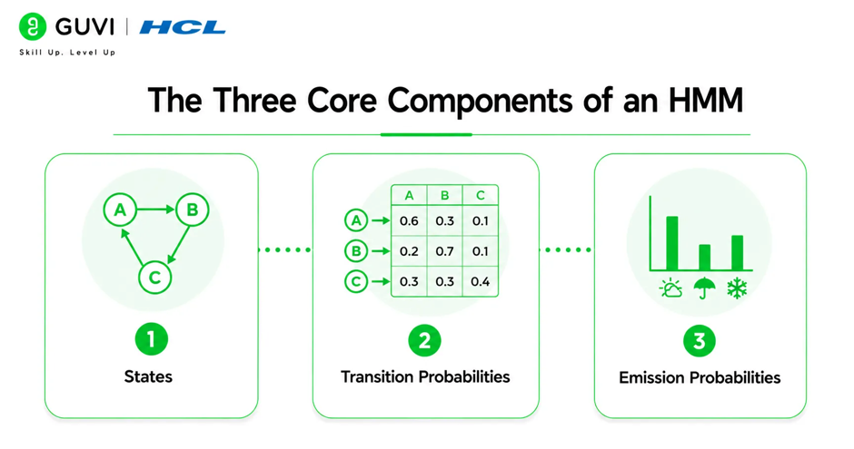
Every Hidden Markov Model is defined by three fundamental components. Understanding these is the foundation for everything else.

1. States

The states are the hidden conditions the system can be in at any given time. You cannot observe them directly. In a speech recognition system, the states might represent different phonemes. In a DNA analysis system, the states might represent different functional regions of a genome such as coding regions and non-coding regions.

The number of states is a design decision you make when building the model, typically based on domain knowledge about the system you are modeling.

2. Transition Probabilities

Transition probabilities describe how likely the system is to move from one state to another at each time step. They are usually represented as a matrix where each row corresponds to the current state and each column corresponds to the next state. Each row sums to one because the system must always move to some state, including the possibility of staying in the same state.

For example, if the system is currently in State A, the transition probabilities might say there is a 70 percent chance of staying in State A and a 30 percent chance of moving to State B.

3. Emission Probabilities

Emission probabilities describe what observable output each hidden state is likely to produce. Each state has its own emission probability distribution. When the system is in a particular state it generates an observation according to that state’s distribution.

For example, if the hidden state represents “Happy”, the emission probabilities might say there is a 60 percent chance of observing the word “great”, a 30 percent chance of “good”, and a 10 percent chance of “okay”. If the hidden state is “Sad”, the emission probabilities would be completely different.

Together, transition probabilities and emission probabilities, along with an initial state distribution, fully define an HMM.

The Three Fundamental HMM Problems

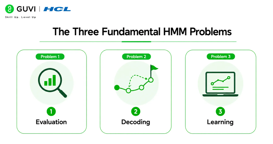
There are three classic problems every HMM practitioner needs to understand. Each one asks a different question about the model and requires a different algorithm to solve.

1. Problem 1: Evaluation

Given a trained HMM and a sequence of observations, what is the probability that this HMM generated that sequence?

This is useful for classification. If you have trained separate HMMs for different speakers, you can evaluate a new observation sequence against all of them and pick the speaker whose HMM assigned the highest probability to that sequence.

The algorithm used to solve this is the Forward Algorithm, which computes the probability efficiently by working through the observation sequence one step at a time and summing over all possible hidden state sequences.

2. Problem 2: Decoding

Given a trained HMM and a sequence of observations, what is the most likely sequence of hidden states that produced those observations?

This is the most intuitive problem. In speech recognition, you observe acoustic signals and want to decode the most likely sequence of words or phonemes. In DNA analysis, you observe a nucleotide sequence and want to decode the most likely sequence of functional regions.

The algorithm used here is the Viterbi Algorithm, which efficiently finds the optimal state sequence using dynamic programming rather than exhaustively checking every possible path.

3. Problem 3: Learning

Given a sequence of observations, how do you find the HMM parameters, meaning the transition and emission probabilities, that best explain those observations?

This is the training problem. You do not know the model parameters upfront. You want to learn them from data.

The algorithm used is the Baum-Welch Algorithm, which is a special case of the expectation-maximization algorithm. It iteratively estimates the hidden states and updates the model parameters until they converge to values that maximize the likelihood of the observed data.

Want to build strong machine learning and statistical modeling skills that apply to real-world data problems? Explore HCL GUVI’s Artificial Intelligence & Machine Learning, designed to help you develop the foundational and advanced ML skills modern data roles demand. 

Conclusion

Hidden Markov Models represent one of the most elegant ideas in statistical machine learning: the recognition that many real-world systems have hidden structure that produces observable evidence, and that you can work backward from what you observe to understand what you cannot see directly. 

The three core components of states, transition probabilities, and emission probabilities, combined with the Forward, Viterbi, and Baum-Welch algorithms, give you a complete toolkit for modeling sequential data with hidden structure.

FAQ