

Artificial Intelligence and Machine Learning Articles
Claude for Product Managers: PRDs and Roadmaps
How to Use Claude for Academic Research


Get In Touch For Details! Request More Information
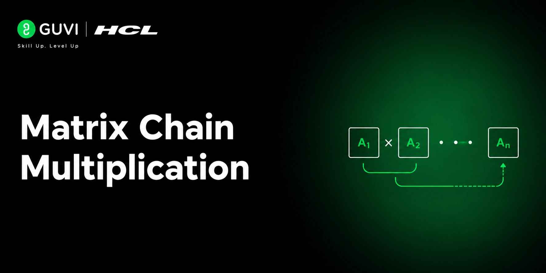
Matrix Chain Multiplication: A Complete Guide
Jul 07, 2026 7 Min Read 954 Views
(Last Updated)
Matrix multiplication is a fundamental operation in computer science, mathematics, and engineering. It underlies everything from computer graphics and machine learning to scientific simulation and signal processing.
When a single pair of matrices must be multiplied, the computation is straightforward. But when a long chain of matrices must be multiplied together, the order in which the multiplications are performed, determined by how the expression is parenthesised, has a dramatic effect on the total number of arithmetic operations required.
This is the matrix chain multiplication problem: given a sequence of matrices, determine the most efficient order to multiply them so that the total number of scalar multiplications is minimised.
It is a classic problem in dynamic programming, taught in every algorithms course because it illustrates the core ideas of optimal substructure and overlapping subproblems with clarity and elegance. This guide explains the problem from first principles, walks through the dynamic programming solution in full, and covers the practical contexts in which matrix chain optimisation matters.
Table of contents
- TL;DR
- Why Parenthesisation Order Matters
- Option 1: (A1 x A2) x A3
- Option 2: A1 x (A2 x A3)
- The Recursive Structure of the Problem
- Optimal Substructure
- Overlapping Subproblems
- The Dynamic Programming Solution
- Notation and Setup
- Algorithm: Bottom-Up DP
- Step-by-Step Worked Example
- Reconstructing the Optimal Parenthesisation
- Time and Space Complexity
- Time Complexity: O(n³)
- Space Complexity: O(n²)
- Comparison with Naive Approaches
- Implementation in Python
- Applications of Matrix Chain Multiplication
- Matrix Chain Multiplication vs. Related Problems
- Conclusion
- FAQs
- What is the matrix chain multiplication problem?
- Why can't we just try all parenthesizations?
- What is the time complexity of the DP solution?
- What do the m and s tables store?
- Where is matrix chain multiplication used in practice?
TL;DR
- Matrix chain multiplication finds the optimal order to multiply a chain of matrices to minimise scalar multiplications.
- The result is the same for all parenthesizations (by associativity), but the computational cost varies widely.
- Naively trying all parenthesizations is exponential; dynamic programming solves it in O(n³) time and O(n²) space.
- The DP approach fills a table m[i][j] storing the minimum cost to multiply matrices from index i to j.
- A separate table s[i][j] records the optimal split point, enabling reconstruction of the optimal parenthesisation.
What Is Matrix Chain Multiplication?
Matrix Chain Multiplication is a classic optimization problem in computer science that determines the most efficient order for multiplying a sequence of matrices. Although matrix multiplication is associative, meaning the final result remains the same regardless of how the matrices are grouped, different parenthesizations can require significantly different numbers of scalar multiplications. The objective is to find the multiplication order that minimizes computational cost rather than performing the actual matrix multiplication. This problem is commonly solved using dynamic programming, achieving a time complexity of O(n³) for a chain of n matrices.
Why Parenthesisation Order Matters

To understand why the problem matters, consider what happens when two matrices are multiplied.
Multiplying an (p x q) matrix by a (q x r) matrix requires exactly p x q x r scalar multiplications and produces a (p x r) result matrix. The dimensions must be compatible: the number of columns in the first matrix must equal the number of rows in the second.
Now consider three matrices:
• A1 : dimensions 10 x 30
• A2 : dimensions 30 x 5
• A3 : dimensions 5 x 60
There are two ways to parenthesise this product: (A1 x A2) x A3 or A1 x (A2 x A3).
Option 1: (A1 x A2) x A3
• Multiply A1 x A2 : cost = 10 x 30 x 5 = 1,500 scalar multiplications. Result: 10 x 5.
• Multiply (10×5) x A3 : cost = 10 x 5 x 60 = 3,000 scalar multiplications.
• Total: 4,500 scalar multiplications.
Option 2: A1 x (A2 x A3)
• Multiply A2 x A3 : cost = 30 x 5 x 60 = 9,000 scalar multiplications. Result: 30 x 60.
• Multiply A1 x (30×60) : cost = 10 x 30 x 60 = 18,000 scalar multiplications.
• Total: 27,000 scalar multiplications.
The second parenthesisation requires six times more computation than the first, yet both produce identical results. For longer chains, the difference can be many orders of magnitude. With a chain of just 10 matrices, the number of possible parenthesizations exceeds 4,000. With 15 matrices, it exceeds 2 billion. An exhaustive search is completely impractical.

The Recursive Structure of the Problem

Before building the dynamic programming solution, it helps to understand the recursive structure of the problem, which reveals both why naive recursion is expensive and why dynamic programming is effective.
Any parenthesisation of a chain A[i..j] (matrices from index i to j) must have a final multiplication at some split point k, where i <= k < j. The left side A[i..k] and the right side A[k+1..j] are each independently parenthesised optimally.
This gives the recursive formulation:
| m[i][j] = 0 if i == jm[i][j] = min over all k from i to j-1 of: m[i][k] + m[k+1][j] + p[i-1] * p[k] * p[j] |
Where p[] is the dimensions array: matrix Ai has dimensions p[i-1] x p[i]. The term p[i-1] * p[k] * p[j] is the cost of the final multiplication that combines the two subchains.
Optimal Substructure
The problem has optimal substructure: an optimal solution to the full problem contains optimal solutions to all its subproblems. If the optimal parenthesisation of A[1..n] splits at position k, then the parenthesisations of A[1..k] and A[k+1..n] within that solution must themselves be optimal. If either subchain were sub-optimally parenthesised, we could improve it and get a better overall solution, a contradiction.
Overlapping Subproblems
The subproblems are not independent. A naive recursive implementation computes the same subproblem, the optimal cost of a given subchain, many times across different branches of the recursion tree. The number of unique subproblems is O(n²), but the naive recursion solves exponentially many total subproblem instances. Memoisation or bottom-up dynamic programming eliminates this redundancy.
The Dynamic Programming Solution

The dynamic programming solution builds a table bottom-up, starting with chains of length 1 and progressively solving longer chains using previously computed shorter-chain results.
Notation and Setup
Given n matrices A1 through An, represent their dimensions as an array p[0..n] where matrix Ai has dimensions p[i-1] x p[i].
Define two tables:
• m[i][j]: The minimum number of scalar multiplications needed to compute the product of matrices Ai through Aj.
• s[i][j]: The index k of the optimal split point that achieves m[i][j] used later to reconstruct the optimal parenthesisation.
Algorithm: Bottom-Up DP
| function MATRIX_CHAIN_ORDER(p[0..n]): n = length(p) – 1 // Base case: single matrices cost zero for i = 1 to n: m[i][i] = 0 // Fill by increasing chain length L for L = 2 to n: // L = chain length for i = 1 to n – L + 1: // i = chain start j = i + L – 1 // j = chain end m[i][j] = INFINITY for k = i to j – 1: // try every split cost = m[i][k] + m[k+1][j] + p[i-1]*p[k]*p[j] if cost < m[i][j]: m[i][j] = cost s[i][j] = k return m, s |
The final answer, the minimum cost to multiply all n matrices, is stored in m[1][n].
Step-by-Step Worked Example
Consider four matrices with dimension array p = [10, 30, 5, 60, 8]:
• A1 : 10 x 30
• A2 : 30 x 5
• A3 : 5 x 60
• A4 : 60 x 8
Step 1 — Base case (chain length L=1): m[i][i] = 0 for all i.
Step 2 — Chain length L=2: compute each adjacent pair.
| m[1][2] = p[0]*p[1]*p[2] = 10*30*5 = 1500 s[1][2] = 1m[2][3] = p[1]*p[2]*p[3] = 30*5*60 = 9000 s[2][3] = 2m[3][4] = p[2]*p[3]*p[4] = 5*60*8 = 2400 s[3][4] = 3 |
Step 3 — Chain length L=3: try all splits for each triple.
| m[1][3]: k=1: m[1][1]+m[2][3]+10*30*60 = 0+9000+18000 = 27000 k=2: m[1][2]+m[3][3]+10*5*60 = 1500+0+3000 = 4500 min = 4500 s[1][3] = 2 m[2][4]: k=2: m[2][2]+m[3][4]+30*5*8 = 0+2400+1200 = 3600 k=3: m[2][3]+m[4][4]+30*60*8 = 9000+0+14400 = 23400 min = 3600 s[2][4] = 2 |
Step 4 — Chain length L=4: compute m[1][4].
| m[1][4]: k=1: m[1][1]+m[2][4]+10*30*8 = 0+3600+2400 = 6000 k=2: m[1][2]+m[3][4]+10*5*8 = 1500+2400+400 = 4300 k=3: m[1][3]+m[4][4]+10*60*8 = 4500+0+4800 = 9300 min = 4300 s[1][4] = 2 |
The minimum cost to multiply all four matrices is 4,300 scalar multiplications, achieved by splitting at k=2: (A1 x A2) x (A3 x A4).
The number of ways to fully parenthesize a chain of n matrices is given by the Catalan number Cn-1, one of the most famous sequences in combinatorics. The count grows explosively: 2 matrices have only 1 valid parenthesization, 4 matrices have 5, 10 matrices have 4,862, and 20 matrices have more than 1.7 billion possible parenthesizations. This rapid growth is why the Matrix Chain Multiplication problem cannot be solved efficiently by brute force. Instead, dynamic programming exploits overlapping subproblems to find the optimal multiplication order in polynomial time, turning a seemingly impossible search problem into a practical algorithm.
Reconstructing the Optimal Parenthesisation
The m table tells us the minimum cost. The s table tells us how to achieve it. Reconstructing the optimal parenthesisation is done by recursively reading the split points stored in s.
| function PRINT_OPTIMAL_PARENS(s, i, j): if i == j: print “A” + i else: print “(” PRINT_OPTIMAL_PARENS(s, i, s[i][j]) PRINT_OPTIMAL_PARENS(s, s[i][j] + 1, j) print “)” |
For our four-matrix example, calling PRINT_OPTIMAL_PARENS(s, 1, 4):
• s[1][4] = 2 → split into A[1..2] and A[3..4].
• s[1][2] = 1 → A[1..1] = A1, A[2..2] = A2. Left subchain: (A1 x A2).
• s[3][4] = 3 → A[3..3] = A3, A[4..4] = A4. Right subchain: (A3 x A4).
• Result: ((A1 x A2) x (A3 x A4))
Time and Space Complexity
Time Complexity: O(n³)
The bottom-up DP algorithm uses three nested loops:
• The outer loop iterates over chain lengths L from 2 to n: O(n) iterations.
• The middle loop iterates over start positions i: O(n) iterations.
• The inner loop iterates over split points k: O(n) iterations.
Total: O(n) x O(n) x O(n) = O(n³). For n = 100 matrices, this is approximately 1,000,000 operations, trivially fast on modern hardware.
Space Complexity: O(n²)
Both the m and s tables are (n+1) x (n+1) square tables. Each store has at most n² values. Total space: O(n²). For n = 1,000 matrices, the tables require approximately 8 MB for 64-bit integers, well within the memory of any modern system.
Comparison with Naive Approaches
- Exhaustive search: O(4^n / n^1.5) exponential. Completely impractical beyond ~20 matrices.
- Naive recursion (no memoisation): O(2^n) exponential due to recomputation of overlapping subproblems.
- Memoised recursion (top-down DP): O(n³) time, O(n²) space, equivalent to bottom-up but with function call overhead.
- Bottom-up DP: O(n³) time, O(n²) space optimal. No recursion overhead.
Implementation in Python
| def matrix_chain_order(p): n = len(p) – 1 # number of matrices # m[i][j] = min cost to multiply A[i..j] m = [[0] * (n + 1) for _ in range(n + 1)] # s[i][j] = optimal split point for A[i..j] s = [[0] * (n + 1) for _ in range(n + 1)] # Base case: single matrix, zero cost # (already 0 from initialisation) # Fill by increasing chain length for length in range(2, n + 1): # chain length for i in range(1, n – length + 2): # start index j = i + length – 1 # end index m[i][j] = float(‘inf’) for k in range(i, j): # split point cost = m[i][k] + m[k+1][j] + p[i-1]*p[k]*p[j] if cost < m[i][j]: m[i][j] = cost s[i][j] = k return m, s def print_optimal_parens(s, i, j): if i == j: print(f”A{i}”, end=””) else: print(“(“, end=””) print_optimal_parens(s, i, s[i][j]) print_optimal_parens(s, s[i][j] + 1, j) print(“)”, end=””) # Example: p = [10, 30, 5, 60, 8]p = [10, 30, 5, 60, 8]m, s = matrix_chain_order(p)print(“Minimum cost:”, m[1][len(p)-1]) # Output: 4300print(“Optimal order: “, end=””)print_optimal_parens(s, 1, len(p)-1) # Output: ((A1A2)(A3A4)) |
Applications of Matrix Chain Multiplication
Matrix chain multiplication is not merely a textbook exercise. The problem of finding an optimal order for a sequence of matrix operations appears throughout applied computing.
- Computer graphics and 3D rendering: Transformation pipelines apply sequences of matrices (translation, rotation, scaling, projection) to every vertex in a scene. Optimising the multiplication order reduces per-frame computation, directly improving frame rate.
- Deep learning and neural networks: Forward and backward passes through neural networks involve multiplying sequences of weight matrices and activation Jacobians. Frameworks like TensorFlow and PyTorch use optimised einsum and contraction ordering to minimise computation.
- Database query optimisation: Relational algebra operations, joins, projections, and selections can be modelled as matrix operations. Optimising their execution order is analogous to matrix chain optimisation and is a central task of query planners.
- Scientific computing: Physics simulations, finite element analysis, and signal processing pipelines involve long chains of matrix operations. Libraries such as NumPy and MATLAB apply optimised ordering strategies automatically.
- Compiler optimisation: Modern compilers optimise sequences of array operations and tensor contractions using techniques directly related to matrix chain ordering, reducing both instruction count and memory bandwidth.
Matrix Chain Multiplication vs. Related Problems
Matrix chain multiplication belongs to a family of interval dynamic programming problems where the state is defined by a contiguous subrange [i, j] of a sequence, and the solution to [i, j] is built from solutions to shorter intervals.
• Optimal binary search tree: Finds the arrangement of keys in a BST that minimises the expected search cost given key access probabilities. Same O(n³) interval DP structure as matrix chain multiplication.
• Burst balloons: A LeetCode problem where coins are collected by bursting balloons in a sequence; the value depends on adjacent elements. Solved with interval DP using the same fill-by-chain-length pattern.
• Polygon triangulation: Finds the minimum-weight triangulation of a convex polygon by decomposing it into triangles structurally identical to matrix chain multiplication with a different cost function.
Recognising the interval DP pattern, try all split points k in [i, j-1], combine subproblem results, and take the minimum is a transferable skill that applies across all of these problems.
If you want practical experience working with activation functions, neural networks, and deep learning models, HCL GUVI’s AI and ML programs can help you understand how concepts like sigmoid, backpropagation, and gradient descent are implemented using frameworks such as TensorFlow and PyTorch through hands-on projects.
Conclusion
Matrix chain multiplication is one of the most instructive problems in the study of dynamic programming. It demonstrates with exceptional clarity why the order of operations matters, how optimal substructure enables a recursive decomposition of a complex problem, and how memoisation or bottom-up table-filling transforms an exponential search into a polynomial-time algorithm.
The O(n³) dynamic programming solution filling the m table by chain length and recording split points in the s table is both elegant and practical. It solves problems that would be computationally intractable with brute force, and the same algorithmic pattern reappears across a wide range of interval optimisation problems.
Beyond the classroom, matrix chain optimisation has direct applications in computer graphics, deep learning, scientific computing, and database systems, anywhere that sequences of matrix operations must be performed efficiently at scale.
Mastering matrix chain multiplication means mastering a way of thinking: decompose by interval, identify the optimal split, and build solutions bottom-up. That thinking is the foundation of dynamic programming itself.
FAQs
1. What is the matrix chain multiplication problem?
Matrix chain multiplication is an optimisation problem that finds the most efficient order to multiply a chain of matrices, minimising the total number of scalar multiplications. The final matrix product is the same regardless of order (associativity), but different parenthesizations have vastly different computational costs.
2. Why can’t we just try all parenthesizations?
The number of distinct parenthesizations of n matrices is the Catalan number C(n-1), which grows exponentially. For n=15, it exceeds 2 billion. Exhaustive search is impractical beyond small chains, making the O(n³) dynamic programming solution essential.
3. What is the time complexity of the DP solution?
The bottom-up dynamic programming algorithm runs in O(n³) time and uses O(n²) space for the m and s tables. It solves all O(n²) subproblems, each requiring O(n) work to find the optimal split point among all candidates.
4. What do the m and s tables store?
The m[i][j] table stores the minimum number of scalar multiplications needed to compute the product of matrices Ai through Aj. The s[i][j] table stores the index k of the optimal split point, enabling reconstruction of the full optimal parenthesisation via traceback.
5. Where is matrix chain multiplication used in practice?
It is used in computer graphics (transformation pipelines), deep learning frameworks (tensor contraction ordering), database query optimisers (join order planning), and scientific computing libraries, anywhere a sequence of matrix operations must be performed at minimum computational cost.
Success Stories

About the Author
Vishalini Devarajan
An Aerospace Engineer turned content writer, I focus on making complex concepts easy to understand through well-structured, reader-friendly blogs. Whether it’s a technical topic or a non-technical one, I love creating content that is clear, engaging, and impactful.
View all posts by Vishalini Devarajan
Connect with me @


Did you enjoy this article?