


Artificial Intelligence and Machine Learning Articles
Generative Adversarial Networks (GANs): The Complete Guide
GRU vs LSTM: Which Should You Use?


Get In Touch For Details! Request More Information
LSTM Networks Explained: Solving the Vanishing Gradient Problem
Aug 26, 2026 4 Min Read 21 Views
(Last Updated)
Imagine trying to predict the next word in a sentence where the key context appeared twenty words earlier. Standard neural networks struggle with this because they process each input independently. Recurrent Neural Networks were designed to handle sequences but developed a crippling weakness: they forget information from too far back because gradients vanish during training. LSTM networks were invented specifically to solve this problem, and they did it so well that they dominated sequential learning tasks for nearly a decade.
Table of contents
- TL;DR Summary
- What Is a Recurrent Neural Network?
- The Vanishing Gradient Problem Explained
- How LSTM Networks Work
- LSTM Gates Summary
- LSTM vs Standard RNN vs GRU
- Implementing LSTM in Python with Keras
- Conclusion
- FAQ
- What is an LSTM network in simple terms?
- What problem do LSTMs solve?
- What are the three gates in an LSTM?
- What is the difference between LSTM and GRU?
- When should I use an LSTM instead of a Transformer?
- How do I choose the sequence length for an LSTM?
TL;DR Summary
- LSTM (Long Short-Term Memory) networks are a special type of recurrent neural network designed to learn long-range dependencies in sequential data
- They solve the vanishing gradient problem that makes standard RNNs fail to learn patterns across long sequences
- An LSTM cell contains three gates: the forget gate, input gate, and output gate, which control what information to keep, add, and use at each time step
- LSTMs are widely used in time series forecasting, natural language processing, speech recognition, and music generation
What Is a Recurrent Neural Network?
A Recurrent Neural Network adds a loop that passes information from one time step to the next. At each step, the network takes the current input and a hidden state from the previous step, combines them, and produces an output plus a new hidden state. This hidden state acts as the network’s memory of what it has seen so far.
In theory, RNNs should be able to learn from arbitrarily long sequences. In practice they fail badly on long sequences because of a problem called the vanishing gradient.
Read More: How to become proficient in deep learning and neural networks
Want to build strong deep learning skills covering LSTMs, neural networks, and real-world sequence modeling? Explore HCL GUVI’s Artificial Intelligence & Machine Learning Course, designed to help you go from ML fundamentals to advanced deep learning applications.
The Vanishing Gradient Problem Explained
Training a neural network uses backpropagation, an algorithm that computes how much each weight contributed to the error and adjusts weights accordingly. For an RNN processing a long sequence, backpropagation must travel back through every time step, multiplying gradients together at each step.
Here is the problem. If those gradients are slightly smaller than 1, multiplying many of them together produces a number that shrinks toward zero exponentially. By the time you reach the early time steps in a long sequence, the gradient has effectively vanished. The weights at those early steps receive almost no update signal, so the network learns nothing about long-range dependencies.
A simple example makes this concrete. Suppose you are training an RNN on the sentence: “The cat, which had been sitting on the mat for several hours, was hungry.” To predict “was hungry” correctly the network needs to remember “The cat” from much earlier. But the vanishing gradient means the signal from those early words becomes negligible by the time it reaches the output, so the network fails to make the connection.
How LSTM Networks Work
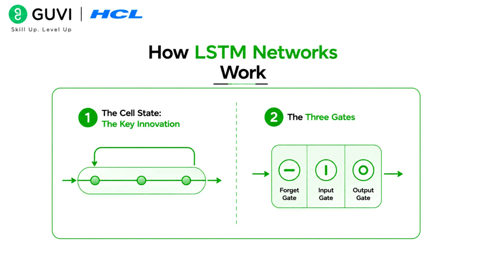
An LSTM network replaces the simple recurrent unit with a more sophisticated memory cell that can maintain information across long sequences without gradients vanishing.
- The Cell State: The Key Innovation
The most important concept in an LSTM is the cell state. Think of it as a conveyor belt running through the entire sequence. Information can be added to or removed from the cell state, but it flows through largely unchanged unless the gates explicitly modify it.
Because the cell state passes through the network with only minor linear interactions, gradients can flow back through many time steps without shrinking to zero. This is what allows LSTMs to learn dependencies across hundreds or even thousands of time steps.
- The Three Gates
LSTMs control what information flows through the cell state using three learnable gates. Each gate is a small neural network that outputs values between 0 and 1. A value of 0 means block everything. A value of 1 means let everything through.
- The Forget Gate decides what information to throw away from the cell state. It looks at the previous hidden state and the current input, and outputs a number between 0 and 1 for each value in the cell state. A value close to 0 means forget this information. A value close to 1 means keep it. For example, when processing a new sentence, the forget gate might clear information about the previous sentence’s subject.
- The Input Gate decides what new information to store in the cell state. It has two parts: a sigmoid layer that decides which values to update, and a tanh layer that creates new candidate values to add. Together they determine what new information enters the cell state. For example, when encountering a new subject in a sentence, the input gate stores information about it to replace what the forget gate cleared.
- The Output Gate decides what to output from the cell state. The cell state is filtered through a tanh function and multiplied by the output gate’s sigmoid output to produce the hidden state that flows to the next time step and to the output layer. This determines what part of the stored memory is actually relevant for the current prediction.
LSTM Gates Summary
| Gate | Question It Answers | Output |
| Forget Gate | What should I forget from memory? | Values between 0 (forget) and 1 (keep) |
| Input Gate | What new information should I store? | New candidate values weighted by importance |
| Output Gate | What should I output right now? | Filtered version of cell state as hidden state |
Hidden Markov Models were first described mathematically by Leonard Baum and colleagues between 1966 and 1972, but remained largely theoretical until the 1980s when researchers at Cambridge and Carnegie Mellon showed they could dramatically improve automatic speech recognition accuracy.

LSTM vs Standard RNN vs GRU
| Feature | Standard RNN | LSTM | GRU |
| Memory mechanism | Hidden state only | Cell state + hidden state | Hidden state only |
| Number of gates | None | 3 (forget, input, output) | 2 (reset, update) |
| Vanishing gradient | Severe problem | Largely solved | Largely solved |
| Parameters | Fewest | Most | Fewer than LSTM |
| Training speed | Fastest | Slowest | Faster than LSTM |
| Long-range dependencies | Poor | Excellent | Good |
| Best for | Very short sequences | Long sequences, complex tasks | Medium sequences, faster training |
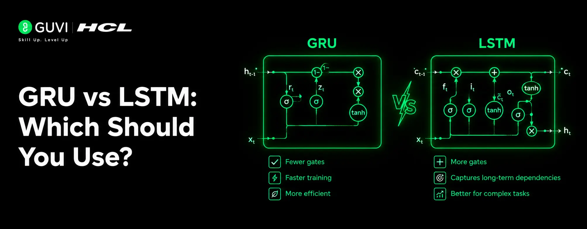
GRU (Gated Recurrent Unit) is a simplified version of LSTM introduced in 2014 that combines the forget and input gates into a single update gate. GRUs train faster and use fewer parameters than LSTMs and perform comparably on many tasks. LSTMs tend to outperform GRUs on tasks requiring very long-range memory.
LSTM networks were invented by Sepp Hochreiter and Jürgen Schmidhuber in 1997, but remained relatively obscure for over a decade due to limited computational resources and datasets. It was not until the deep learning revival around 2012 to 2014, combined with GPU acceleration and large datasets, that LSTMs achieved their breakthrough results in speech recognition, machine translation, and language modeling that made them famous.
Implementing LSTM in Python with Keras
Keras makes LSTM implementation straightforward. Here is a complete example for time series prediction:
import numpy as np

from tensorflow.keras.models import Sequential

from tensorflow.keras.layers import LSTM, Dense

from sklearn.preprocessing import MinMaxScaler

scaler = MinMaxScaler()

data_scaled = scaler.fit_transform(data.reshape(-1, 1))

def create_sequences(data, seq_length):

    X, y = [], []

    for i in range(len(data) - seq_length):

        X.append(data[i:i + seq_length])

        y.append(data[i + seq_length])

    return np.array(X), np.array(y)

seq_length = 30

X, y = create_sequences(data_scaled, seq_length)

split = int(len(X) * 0.8)

X_train, X_test = X[:split], X[split:]

y_train, y_test = y[:split], y[split:]

model = Sequential([

    LSTM(50, activation="tanh", return_sequences=False,

         input_shape=(seq_length, 1)),

    Dense(1)

])

model.compile(optimizer="adam", loss="mse")

model.fit(X_train, y_train, epochs=50, batch_size=32,

          validation_data=(X_test, y_test), verbose=1)
The input shape for an LSTM layer is always (timesteps, features). The return_sequences parameter controls whether the LSTM returns output at every time step (True, needed when stacking LSTM layers) or only at the final time step (False, used for prediction tasks).
Conclusion
LSTM networks solved one of the fundamental problems in sequential deep learning by introducing a cell state and gating mechanism that allows gradients to flow across long sequences without vanishing.
Their impact on speech recognition, machine translation, and time series modeling through the 2010s was transformative, and their relevance continues in 2026 for applications where efficiency, sequential processing, and strong performance on numerical time series matter more than raw NLP benchmark scores.
FAQ
What is an LSTM network in simple terms?
An LSTM is a type of recurrent neural network with a special memory mechanism that allows it to learn patterns across long sequences by controlling what information to keep, add, and use at each time step.
What problem do LSTMs solve?
LSTMs solve the vanishing gradient problem that makes standard RNNs fail to learn dependencies between inputs that are far apart in a sequence.
What are the three gates in an LSTM?
The forget gate decides what to remove from memory. The input gate decides what new information to store. The output gate decides what to pass to the next time step and the output layer.
What is the difference between LSTM and GRU?
GRU is a simplified version of LSTM with two gates instead of three and no separate cell state. GRUs train faster with fewer parameters and perform comparably to LSTMs on many tasks. LSTMs tend to outperform GRUs on tasks requiring very long-range memory.
When should I use an LSTM instead of a Transformer?
Use LSTMs for time series forecasting, real-time sequential prediction, embedded systems with constrained resources, and long sequences where Transformer quadratic scaling becomes computationally impractical.
How do I choose the sequence length for an LSTM?
Use domain knowledge about your problem. If you are forecasting monthly sales and suspect seasonal patterns, use a sequence length of at least 12. If you are processing text, common choices are 50 to 200 tokens depending on the typical document length in your dataset.
Success Stories

About the Author
HCL GUVI
This article was selected and published as part of the HCL GUVI AI Blogathon 2026, an initiative designed to encourage students, AI enthusiasts, and aspiring tech writers to simplify complex AI concepts through impactful technical content. The contest recognized high-quality, original, and insightful AI-focused blogs, with selected authors receiving publication opportunities on the HCL GUVI blog platform along with official author credits and recognition.
View all posts by HCL GUVI
Connect with me @









Did you enjoy this article?