Generalized Linear Models (GLM): A Guide for Beginners

Have you ever wondered why linear regression alone isn’t enough to model the real world? Imagine you’re trying to predict whether a person has a disease (yes/no) or how many customers might visit your store on a weekend. A straight-line equation won’t cut it here,  because the outcome isn’t always continuous and numeric.

That’s where Generalized Linear Models (GLMs) step in. GLMs extend the familiar linear regression framework so you can handle binary outcomes, counts, proportions, and much more,  all while keeping the core “linear” idea intact.

In this article, we’ll break down GLMs in a way that’s both approachable and mathematically grounded. So, without further ado, let us get started!

What is a Generalized Linear Model?

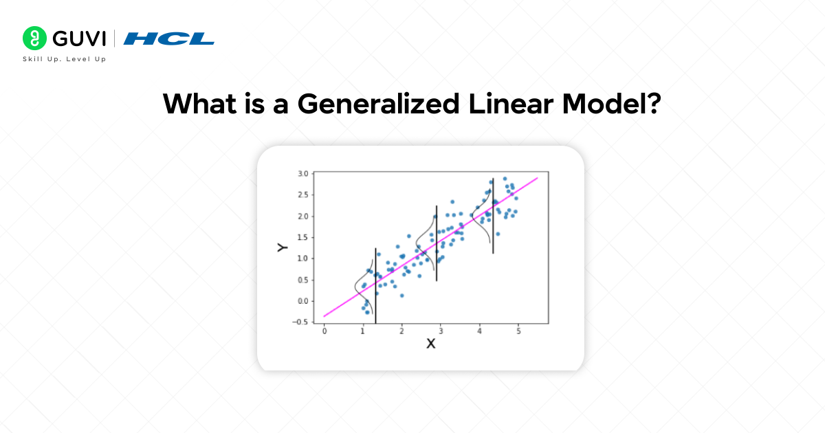
Here’s the thing: linear regression is great when your target is continuous, roughly normal, and the variance doesn’t change with the mean. Real data rarely behaves that nicely. 

At its core, a GLM is a framework for predicting outcomes that don’t fit neatly into the “straight line + normal errors” assumption of traditional regression.

Here’s what makes GLMs different:

• They work with many types of outcomes. Not just continuous numbers, but also binary (yes/no), counts (0, 1, 2, …), or skewed positive values.
  
• They use special transformations, called link functions. These functions connect the predictors to the outcome in a way that makes sense for that type of data.
  
• They keep the regression idea alive. You still linearly combine predictors, but the link function helps map that linear predictor onto outcomes that fit reality.

Think of GLMs as a flexible toolkit: instead of trying to force every dataset into a straight-line model, you pick the right distribution and link function for the job. 

Components of a Generalized Linear Model

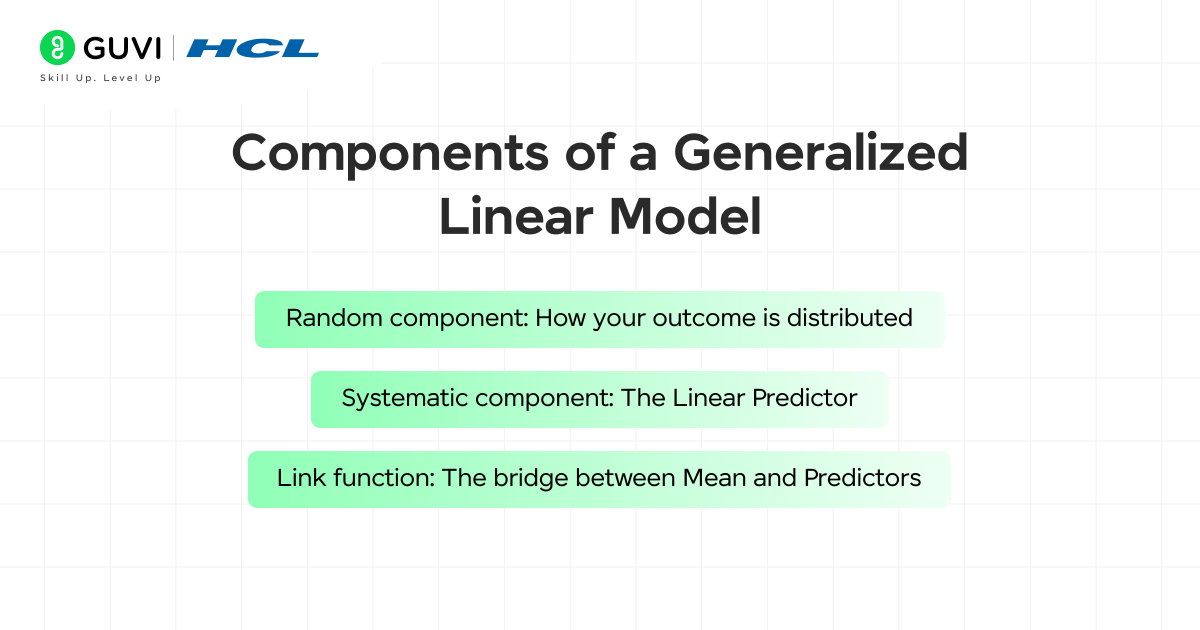
GLMs keep the familiar regression backbone but swap in smarter pieces so the model fits the data you actually have. Think of it as three parts that click together.

1) Random component: How your outcome is distributed

This is the “data-generating story.” You choose a probability distribution that matches the kind of outcome you’re predicting.

• Normal: For continuous outcomes centered around a mean with roughly constant spread (e.g., test scores, heights).
  
• Binomial: For binary outcomes (yes/no) or proportions (successes out of trials).
  
• Poisson: For counts that are non-negative and often “rarer” events (visits, calls, defects).
  
• Gamma: For positive, right-skewed values (costs, waiting times).
  
• Inverse Gaussian: Also positive and skewed, useful for some time-to-event data.

Why it matters: The distribution dictates how variance behaves. For example, Poisson variance grows with the mean, while binomial variance depends on the success probability. If your residuals look off or your uncertainty is understated, your distribution might be wrong.

2) Systematic component: The Linear Predictor

All predictors feed in linearly to form a single score (the linear predictor). Even when the outcome behaves nonlinearly on its own scale, the relationship is linear after you apply the link function (next section).

What to include:

• Main effects: Your core features (age, price, time on site).
  
• Interactions: When the effect of one feature depends on another (e.g., discount works differently on weekends).
  
• Nonlinear terms: Polynomials or splines to capture curvature while staying in the GLM family.
  
• Categoricals: One-hot or effect coding to represent categories cleanly.

Interpretation lives here. Coefficients tell you the direction and size of effects on the link scale. Convert them back to a more natural scale (odds, rates, or percent changes) when explaining results.

3) Link function: The bridge between the Mean and the Predictors

The link function maps the model’s linear predictor to the expected outcome in a way that respects the outcome’s bounds.

• Identity: Keeps values as-is (typical for Normal).
  
• Logit: Maps probabilities to the real line and back to 0–1 (typical for Binomial).
  
• Log: Keeps predicted means positive and turns multiplicative effects into additive ones on the log scale (typical for Poisson and often for Gamma).
  
• Probit / complementary log-log: Alternatives to logit with different tail behavior (handy in some risk or time-to-event contexts).

How to choose:

• Respect the support (probabilities must stay in 0–1, counts must be ≥ 0).
  
• Pick for interpretability (logit → odds ratios; log → rate ratios or percentage changes).
  
• Validate with diagnostics (residual plots, information criteria, calibration checks).

Types of GLMs

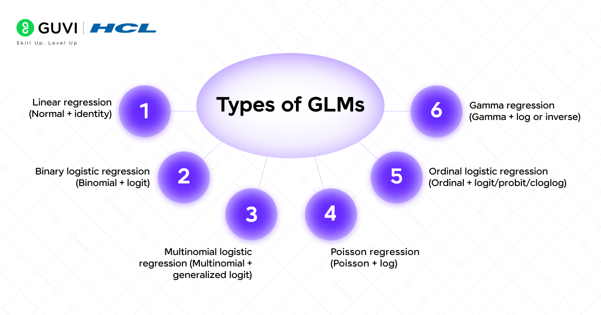
Each “type” is just a sensible pairing of distribution + link, with the linear predictor doing the heavy lifting. Here are the ones you’ll use most, plus when and why.

1) Linear regression (Normal + identity)

Use when your outcome is continuous, roughly symmetric, and the spread doesn’t change much across the range.

Interpretation: A one-unit change in a predictor shifts the expected outcome by a fixed amount.

Example: Predicting the monthly electricity bill from square footage and appliances.

2) Binary logistic regression (Binomial + logit)

Use when the outcome is yes/no or a proportion.

Interpretation: Coefficients become odds ratios after exponentiation. Easy to communicate (“2× the odds”).

Example: Likelihood of a user signing up after a trial; disease presence vs absence.

3) Multinomial logistic regression (Multinomial + generalized logit)

Use when there are more than two categories with no natural order (A/B/C choices).

Interpretation: Effects relative to a reference class.

Example: Predicting which subscription tier a user chooses.

4) Ordinal logistic regression (Ordinal + logit/probit/cloglog)

Use when categories have a natural order (e.g., low/medium/high).

Interpretation: How predictors shift the odds of being in a higher category.

Example: Credit ratings, pain scales, customer satisfaction levels.

5) Poisson regression (Poisson + log)

Use when the response is a count and the variance scales with the mean. Often includes an offset for exposure time or population.

Interpretation: Exponentiated coefficients are rate ratios (percent change in expected count).

Example: Number of support tickets per day, incidents per 1000 users.

6) Gamma regression (Gamma + log or inverse)

Use when the outcome is positive and right-skewed (costs, durations).

Interpretation: With a log link, coefficients read as multiplicative effects (e.g., +10% cost).

Example: Claim amounts, length of hospital stay, time to complete a task.

How Generalized Linear Models Work in Practice?

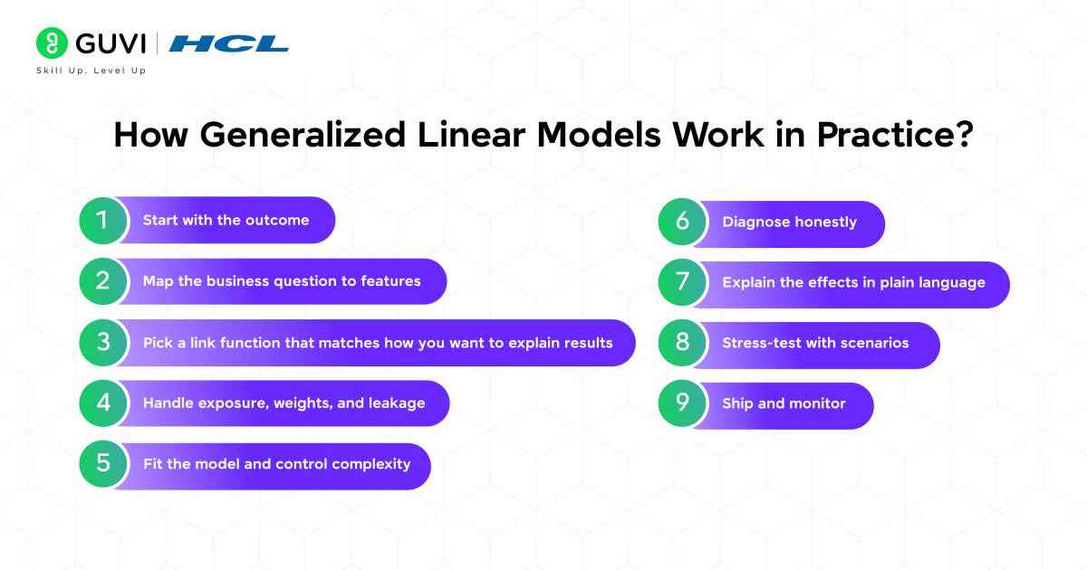
GLMs feel intimidating until you see the workflow. After that, it’s a repeatable playbook you can run across projects.

1) Start with the outcome

First ask: what are you predicting?

• A yes/no event (purchase, dropout, disease) → think logistic (binomial).
  
• A count (visits, tickets, claims) → start with Poisson, check if you need negative binomial.
  
• A positive, skewed value (costs, time spent, length of stay) → Gamma (often with a log link).
  
• A continuous value that can go up or down → linear regression (normal).

This choice aligns the model with how the data behave. It keeps predictions valid (no negative counts, no probabilities beyond 0–1).

2) Map the business question to features

List the drivers that plausibly influence the outcome. Make them measurable.

• Use domain logic: “more sessions → higher chance of purchase.”
  
• Encode categories cleanly (one-hot or effects coding).
  
• Add interactions only where they make sense (“discount × weekend”).
  
• For curvature, use splines/polynomials rather than forcing an ML jump.

Tip: document each feature’s “why.” It helps later when you justify the model.

3) Pick a link function that matches how you want to explain results

• Logit for probabilities (odds ratios are easy to communicate).
  
• Log for counts and positive outcomes (interpret as rate or percent change).
  
• Identity when differences in original units matter.

Choose the link you can explain to a stakeholder in one sentence.

4) Handle exposure, weights, and leakage

• Offsets: If you’re modeling rates, add exposure as an offset (e.g., time at risk, population, pageviews). This keeps comparisons fair.
  
• Weights: Use them for aggregated rows (e.g., successes out of trials) or to correct sampling.
  
• Leakage: Exclude features that wouldn’t be known at prediction time (refund reason, future usage).

5) Fit the model and control complexity

• Start simple. Add complexity only when it clearly improves fit or interpretability.
  
• If separation or instability appears in logistic models, add regularization (L1/L2) or simplify predictors.
  
• For high variance or rare events, try class-balanced sampling, penalized likelihood, or Firth correction (conceptually: shrink the extremes).

6) Diagnose honestly

You don’t need formulas to know if a GLM is lying to you. Look for:

• Calibration (for probabilities): predicted 0.7 should happen about 70% of the time.
  
• Discrimination: ROC-AUC/PR-AUC for binary; for counts or costs, compare predicted vs. observed across quantiles.
  
• Overdispersion: for counts/proportions, if residual variability is larger than the model expects, move to negative binomial or quasi families.
  
• Residual patterns: strong structure means a missing feature, wrong link, or wrong family.
  
• Information criteria (AIC/BIC): lower is usually better when comparing reasonable alternatives.

7) Explain the effects in plain language

Translate coefficients on the link scale into something human:

• Logistic: “This factor doubles the odds of conversion.”
  
• Poisson/NegBin: “A one-unit increase leads to ~12% more tickets on average.”
  
• Gamma (log link): “This segment has ~18% higher cost holding others constant.”
  
• Linear: “Adds about ₹1,200 to the expected bill.”

Prefer marginal effects or predicted scenarios over raw coefficients when presenting to non-statisticians.

8) Stress-test with scenarios

Change one input while holding others fixed and see what the model says. Useful checks:

• Are predictions realistic at extremes?
  
• Does the model react sensibly to business-critical levers (price, time on site)?
  
• Are there thresholds where policy changes would flip a decision?

9) Ship and monitor

• Logging: store inputs, predictions, and (later) outcomes.
  
• Drift: watch for shifts in feature distributions or outcome rates.
  
• Recalibration: if probabilities drift, recalibrate or refit on recent data.
  
• Governance: version the model, record assumptions, document limitations.

That’s the loop: choose the family, build a sensible linear predictor, link it properly, check fit, translate effects, and keep the model honest in production.

Real-World Applications of GLMs

GLMs show up everywhere:

• Healthcare: Predicting disease occurrence (yes/no), modeling hospital stays, or patient readmission counts.
  
• Finance & Insurance: Estimating loan default probability, predicting insurance claim frequency, or modeling claim costs.
  
• Marketing: Estimating click-through rates for ads, predicting customer churn, or analyzing A/B test results.
  
• Engineering: Modeling machine failure times or the number of defects in a production line.
  
• Environmental Science: Modeling species counts in an ecosystem, or the probability of extreme weather events.

If you’ve used logistic regression in a project, you’ve already used a GLM.

Advantages of GLMs

Why use GLMs instead of sticking with linear regression or jumping to complex machine learning?

• Flexibility: Can handle binary, count, proportion, or skewed continuous data.
  
• Unified framework: Different models (logistic, Poisson, gamma) all follow the same structure, so once you know one, you can learn the rest quickly.
  
• Interpretability: Results are easier to explain — odds ratios, rate ratios, or percent changes are intuitive for decision-making.
  
• Software support: Available in R, Python, SAS, SPSS, and nearly every analytics tool.
  
• Foundation for advanced models: GLMs are stepping stones to more advanced methods like Generalized Additive Models (GAMs) and Generalized Linear Mixed Models (GLMMs).

Limitations of GLMs

GLMs are powerful, but they aren’t perfect. Some limitations include:

• Model specification matters: You need to choose the right distribution and link. The wrong choice can lead to poor results.
  
• Linearity assumption: GLMs assume predictors relate linearly to the outcome on the link scale. Real-world data may require extra transformations.
  
• Sensitivity to outliers: A few unusual data points can skew the results.
  
• Not ideal for very complex structures: For hierarchical or highly non-linear data, GLMMs or machine learning methods may be better.
  
• Overdispersion issues: Especially in Poisson regression, where data has more variability than the model allows.

If you’re serious about mastering Machine Learning concepts like GLMs and want to apply them in real-world scenarios, don’t miss the chance to enroll in HCL GUVI’s Intel & IITM Pravartak Certified Artificial Intelligence & Machine Learning Course. Endorsed with Intel certification, this course adds a globally recognized credential to your resume, a powerful edge that sets you apart in the competitive AI job market.

Conclusion

In conclusion, Generalized Linear Models extend linear regression into a powerful family of models that can handle binary outcomes, counts, proportions, and skewed data. 

By understanding their components,  distribution, linear predictor, and link function, you unlock the ability to model a wide range of real-world problems.

The next time you face data that doesn’t fit into a straight line, remember: a GLM might be the right tool for you.

FAQs 

1. What is the difference between GLM and linear regression?

Linear regression is just one special case of GLM, meant for continuous outcomes. GLMs extend this idea to handle binary, count, and skewed data.

2. Why do we use GLMs?

Because not all outcomes are continuous and normal. GLMs give you a way to model outcomes that better reflect reality.

3. What are some real-world examples of GLMs?

Predicting disease risk (logistic), modeling insurance claims (Poisson), and estimating costs (gamma).

4. What is a link function in GLMs?

It’s the transformation that connects predictors to the outcome in a way that respects the outcome’s range (like keeping probabilities between 0 and 1).

5. What are the limitations of GLMs?

They require careful choice of distribution and link, can be sensitive to outliers, and don’t handle very complex data structures on their own.