


Artificial Intelligence and Machine Learning Articles
Generative Adversarial Networks (GANs): The Complete Guide
GRU vs LSTM: Which Should You Use?
LSTM Networks Explained: Solving the Vanishing Gradient Problem


Get In Touch For Details! Request More Information
Seasonal Decomposition of Time Series Explained
Aug 26, 2026 4 Min Read 22 Views
(Last Updated)
Time series data often contains several patterns at once. A company’s sales might steadily increase over several years while also rising every weekend or during particular seasons. Seasonal Decomposition helps analysts separate these patterns so they can better understand what is happening within the data.
Instead of examining a time series as one continuous sequence, decomposition breaks it into meaningful components such as trend, seasonality, and residual variation. This makes it useful for forecasting, anomaly detection, business analysis, and exploratory data analysis.
Table of contents
- TL;DR
- What Is Seasonal Decomposition?
- Why Is Seasonal Decomposition Important?
- The Main Components of a Time Series
- Additive vs Multiplicative Decomposition
- How Does Seasonal Decomposition Work?
- Seasonal Decomposition with Python
- What Is STL Decomposition?
- Seasonal Decomposition for Forecasting
- Seasonal Decomposition for Anomaly Detection
- A Simple Example
- Key Takeaways
- Conclusion
- FAQs
- What is Seasonal Decomposition?
- What are the three main components of decomposition?
- What is the difference between additive and multiplicative decomposition?
- What is STL decomposition?
- Can Seasonal Decomposition be used for forecasting?
TL;DR
- Seasonal Decomposition separates a time series into trend, seasonal, and residual components.
- It helps identify recurring patterns and long-term movement.
- Additive and multiplicative decomposition are two common approaches.
- Methods such as classical decomposition and STL can be used in practice.
- Decomposition is useful for forecasting, anomaly detection, and understanding time-dependent data.
What Is Seasonal Decomposition?
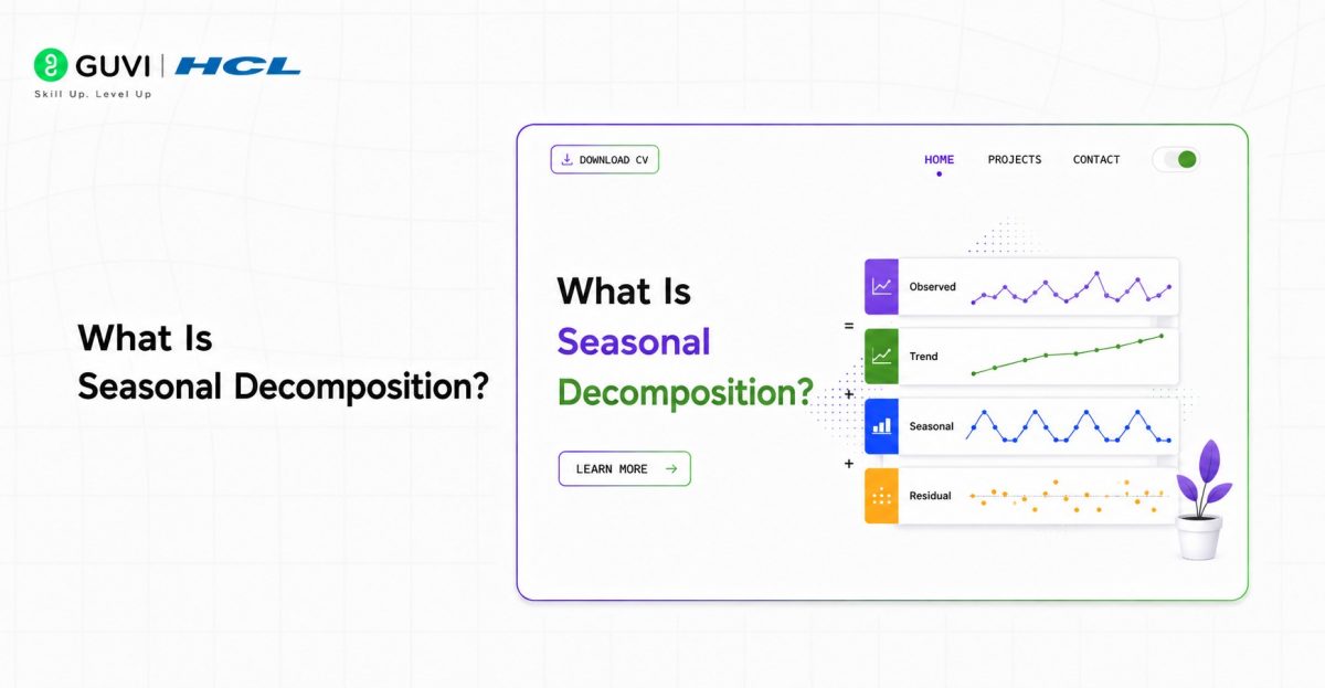
Seasonal Decomposition is a time series analysis technique that breaks observed data into separate components.
A typical decomposition contains:
- Trend: The long-term direction of the series.
- Seasonality: A repeating pattern occurring at a known frequency.
- Residual: Variation that remains after the trend and seasonal components are removed.
A simplified additive model is:
Observed = Trend + Seasonal + ResidualFor example, consider monthly retail sales. The trend may show gradual business growth, while the seasonal component may reveal that sales consistently increase during certain months.
Read More: Core Data Science Concepts Every Beginner Must Know in 2026
Build practical AI and ML skills with HCL GUVI’s Artificial Intelligence & Machine Learning Course. Learn time series analysis, machine learning, and predictive techniques through real-world projects.
Why Is Seasonal Decomposition Important?
Looking only at the original time series can make it difficult to distinguish long-term trends from recurring seasonal effects.
Decomposition allows you to ask more specific questions:
- Is the business actually growing?
- Are sales increasing only because of seasonal demand?
- Which periods consistently perform better?
- Are there unusual observations that do not fit the normal pattern?
This makes decomposition valuable before building a forecasting model.
Seasonal patterns can occur at different frequencies. Depending on the data, you might observe yearly, quarterly, monthly, weekly, or even daily patterns.
The Main Components of a Time Series
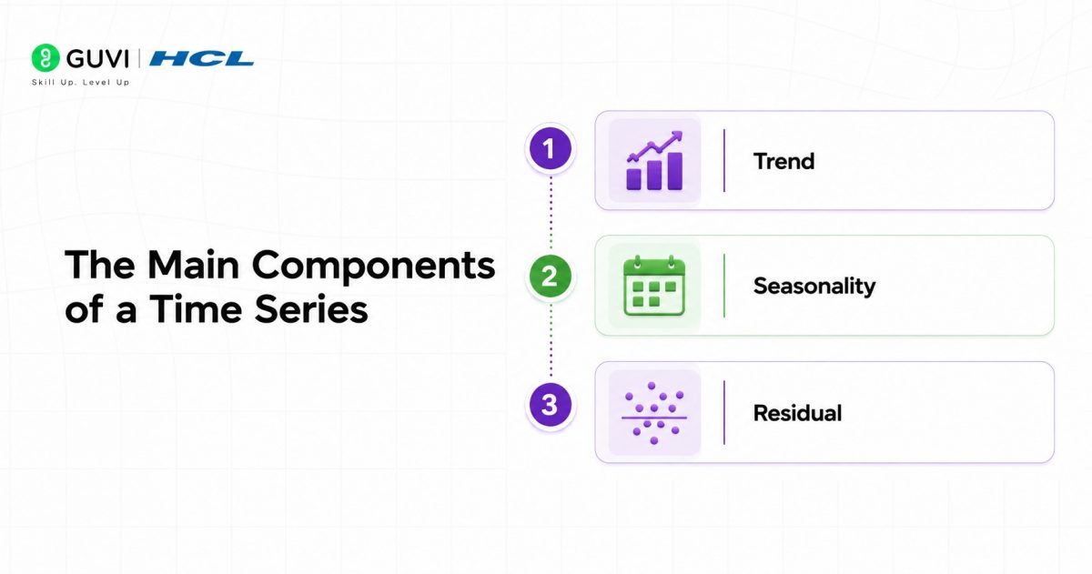
- Trend
The trend represents the long-term movement of the data.
For example, a company’s revenue might increase gradually over several years. Even though individual months fluctuate, the overall direction may remain upward.
Trend analysis helps identify whether a series is generally:
- Increasing
- Decreasing
- Stable
- Changing direction
- Seasonality
Seasonality represents a pattern that repeats at a predictable frequency.
Examples include:
- Higher retail sales during holidays
- Increased electricity demand during particular seasons
- Weekly website traffic patterns
- Monthly subscription cycles
The key characteristic is repetition at a known interval.
- Residual
The residual component contains variation that is not explained by the estimated trend and seasonal patterns.
Residuals may represent:
- Random fluctuations
- Unexpected events
- Measurement errors
- Anomalies
- Patterns not captured by the decomposition model
Pro Tip: Inspect residuals after decomposition. If strong patterns remain, your chosen model may not be capturing all of the important structure in the data.
Additive vs Multiplicative Decomposition
Two common decomposition models are additive and multiplicative.
- Additive Decomposition
An additive model assumes that the size of the seasonal effect remains relatively constant over time.
Y(t) = T(t) + S(t) + R(t)For example, if sales consistently increase by approximately 500 units every December, an additive model may be appropriate.
- Multiplicative Decomposition
A multiplicative model assumes that seasonal effects change proportionally with the level of the series.
Y(t) = T(t) × S(t) × R(t)For example, if December sales are consistently around 30% higher than the normal level, a multiplicative model may better represent the pattern.
| Characteristic | Additive | Multiplicative |
| Seasonal effect | Relatively constant | Changes with series level |
| Relationship | Sum of components | Product of components |
| Suitable for | Stable seasonal variation | Proportional seasonal variation |
Best Practice: Plot the original series before selecting a decomposition type. If seasonal fluctuations become larger as the overall series grows, multiplicative behavior may be more appropriate.
How Does Seasonal Decomposition Work?
A typical decomposition workflow looks like this:
- Collect and organize time series data.
- Ensure observations have a consistent time frequency.
- Identify the likely seasonal period.
- Estimate the trend.
- Extract the seasonal component.
- Calculate the residual component.
- Analyze each component separately.
The process transforms a complex time series into simpler patterns that can be interpreted independently.
Seasonal Decomposition with Python
Python provides several tools for performing decomposition. One commonly used approach is available through statsmodels.
from statsmodels.tsa.seasonal import seasonal_decompose

result = seasonal_decompose(

    df["sales"],

    model="additive",

    period=12

)

result.plot()
For monthly data with yearly seasonality, a period of 12 is commonly used.

For weekly data with a weekly cycle, a different period would be appropriate.
The correct period depends on the frequency and behavior of your dataset.
What Is STL Decomposition?
STL, or Seasonal-Trend decomposition using Loess, is a more flexible decomposition technique.
It uses locally weighted regression to estimate the trend and seasonal components. Compared with classical decomposition, STL can provide greater flexibility when the trend changes over time.
STL can also be useful when the time series contains unusual observations.
A Python implementation can be created using:
from statsmodels.tsa.seasonal import STL

result = STL(

    df["sales"],

    period=12

).fit()

result.plot()
Warning: STL and other decomposition techniques still depend on choosing an appropriate seasonal period. An incorrect period can produce misleading components.
Seasonal Decomposition for Forecasting
Decomposition can be useful as part of a forecasting workflow.
A common process is:
Historical Data → Decomposition → Pattern Analysis → Forecasting Model → PredictionsFor example, an analyst might discover that a company’s sales contain:
- Strong upward trend
- Consistent yearly seasonality
- Several unusual spikes
This information can help guide the selection and configuration of a forecasting model.
However, decomposition itself does not automatically produce future predictions.
Seasonal Decomposition for Anomaly Detection
Residuals can also help identify unusual observations.
Suppose a company’s sales normally follow a predictable seasonal pattern. If one month has a much larger residual than expected, it could indicate an unusual event.
Possible explanations include:
- A successful marketing campaign
- Supply problems
- Extreme weather
- Data collection errors
- Unexpected customer behavior
Data Point: Decomposition can make anomalies easier to detect because unusual observations can be evaluated after removing expected trend and seasonal effects.
A Simple Example
Imagine a company tracking monthly sales for five years.
The raw data shows fluctuations that make the overall pattern difficult to interpret.
After decomposition, the company discovers:
- Trend: Sales have increased steadily.
- Seasonality: Sales rise every December.
- Residual: A few months contain unusually large spikes.
This gives the business a much clearer understanding of its historical performance and provides useful information for future forecasting.
Key Takeaways
- Seasonal Decomposition separates time series into trend, seasonal, and residual components.
- Additive decomposition works when seasonal effects remain relatively constant.
- Multiplicative decomposition is useful when seasonal effects change proportionally with the series level.
- STL provides a flexible alternative for decomposition.
- Residuals can help identify unusual observations.
- Choosing the correct seasonal period is essential.
- Decomposition helps analysis but does not automatically create forecasts.
Conclusion
Seasonal Decomposition provides a practical way to understand the hidden structure of time series data. By separating long-term trends, recurring seasonal patterns, and unexplained variation, analysts can interpret complex datasets more effectively.
Whether you’re analyzing sales, website traffic, energy consumption, or other time-dependent measurements, decomposition can be a valuable first step before forecasting or anomaly detection. The key is to choose an appropriate decomposition method and seasonal period while carefully validating whether the resulting components make sense for the real-world problem.
FAQs
What is Seasonal Decomposition?
Seasonal Decomposition is a time series technique that separates observed data into trend, seasonal, and residual components.
What are the three main components of decomposition?
The three main components are trend, seasonality, and residual variation.
What is the difference between additive and multiplicative decomposition?
Additive decomposition assumes relatively constant seasonal effects, while multiplicative decomposition models seasonal effects that change proportionally with the level of the series.
What is STL decomposition?
STL, or Seasonal-Trend decomposition using Loess, is a flexible method that uses locally weighted regression to estimate trend and seasonal components.
Can Seasonal Decomposition be used for forecasting?
Yes. Decomposition can help identify patterns that inform forecasting, although decomposition itself is primarily an analysis technique rather than a complete forecasting model.
Success Stories

About the Author
HCL GUVI
This article was selected and published as part of the HCL GUVI AI Blogathon 2026, an initiative designed to encourage students, AI enthusiasts, and aspiring tech writers to simplify complex AI concepts through impactful technical content. The contest recognized high-quality, original, and insightful AI-focused blogs, with selected authors receiving publication opportunities on the HCL GUVI blog platform along with official author credits and recognition.
View all posts by HCL GUVI
Connect with me @











Did you enjoy this article?