


Data Science Articles
Hypothesis Testing: A Beginner's Guide for Data Scientists
Pandas Advanced Techniques for Data Scientists
Data Warehouse vs. Data Lake vs. Lakehouse: What's the Difference?
SQL Window Functions: Practical Examples Every Analyst Needs


Get In Touch For Details! Request More Information
Decision Tree in Data Science: Working, Algorithms, Python, and Applications
Oct 01, 2026 12 Min Read 4435 Views
(Last Updated)
Decision Trees are among the most interpretable supervised machine learning algorithms used in Data Science. They convert a prediction problem into a sequence of feature-based rules, making it possible to trace exactly how the model reaches a classification or regression output.
A Decision Tree repeatedly splits a dataset into smaller subsets using conditions such as Age <= 30 or Income > 50000. The algorithm selects each split by measuring how effectively it separates the target variable.
Decision Trees are useful not only as standalone models but also as the foundation of powerful ensemble algorithms such as Random Forest and Gradient Boosting.
This guide explains how Decision Trees work in Data Science, how split criteria such as Gini Impurity and Entropy are calculated, how pruning controls overfitting, how important hyperparameters affect model behaviour, and how to build and evaluate a Decision Tree using Python.
Table of contents
- Quick Answer
- What Is a Decision Tree in Data Science?
- Decision Tree Classification vs Regression
- Key Features of Decision Trees in Data Science
- How Decision Trees Choose the Best Split
- Entropy and Information Gain
- Gini Impurity vs Entropy
- How Regression Trees Select Splits
- Key Applications of Decision Trees in Data Science
- Fraud Detection
- Customer Churn Prediction
- Credit Risk Assessment
- Sales and Demand Prediction
- Customer Segmentation Rules
- Operational Risk and Predictive Maintenance
- Advantages of Decision Trees in Data Science
- Highly Interpretable
- Handles Nonlinear Relationships
- Does Not Require Feature Scaling
- Supports Classification and Regression
- Captures Feature Interactions
- Can Provide Feature Importance
- How Decision Trees Work
- Root Node Starts With the Complete Dataset
- The Algorithm Evaluates Candidate Splits
- The Best Split Becomes an Internal Node
- Branches Represent Split Outcomes
- Recursive Partitioning Continues
- Leaf Nodes Produce Final Predictions
- Tree Growth Stops Based on Defined Conditions
- Prediction Follows One Root-to-Leaf Path
- Classification and Regression Trees Use Different Split Objectives
- Pruning Controls Overfitting
- Decision Tree Example: How a Prediction Is Made
- Implementing Decision Trees in Data Science: Step-by-Step
- Step 1: Import the Required Libraries
- Step 2: Load and Inspect the Dataset
- Step 3: Split the Data Into Training and Test Sets
- Step 4: Configure the Decision Tree Model
- Step 5: Train the Decision Tree
- Step 6: Generate Predictions
- Step 7: Evaluate Model Performance
- Step 8: Visualize the Decision Tree
- Step 9: Examine Feature Importance
- Step 10: Tune the Decision Tree
- Step 11: Use Decision Trees for Regression
- Complete Decision Tree Workflow
- Decision Tree vs Random Forest vs Gradient Boosting
- Common Mistakes When Building Decision Trees
- Training and Testing on the Same Dataset
- Allowing Unlimited Tree Growth
- Evaluating Only Accuracy
- Treating Feature Importance as Causality
- Ignoring Class Imbalance
- Using a Very Small Toy Dataset as Proof of Performance
- How to Improve Decision Tree Performance
- When Should You Use a Decision Tree?
- Decision Trees in Modern Data Science
- Limitations of Decision Trees
- Overfitting
- Model Instability
- Greedy Split Selection
- Poor Extrapolation in Regression
- Deep Trees Lose Interpretability
- Impurity-Based Feature Importance Can Mislead
- Conclusion
- FAQs
- Q1. Do I need coding for data science?
- Q2. Is DSA required for data science?
- Q3. Which language is best for data science?
- Q4. What industries hire data scientists?
- Q5. Is data science a good career for freshers
Quick Answer
A Decision Tree in Data Science is a supervised machine learning algorithm that recursively divides data using feature-based conditions until it reaches a prediction at a leaf node.
- Classification: Predicts categories such as fraud vs legitimate or churn vs retained.
- Regression: Predicts continuous values such as sales, demand, or house prices.
- Split Criteria: Classification commonly uses Gini Impurity or Entropy, while regression can use squared error.
- Main Strength: Produces human-readable decision rules without requiring feature scaling.
- Main Limitation: Deep trees can overfit training data and become unstable.
What Is a Decision Tree in Data Science?
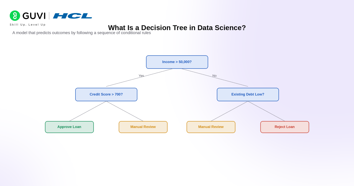
A Decision Tree is a supervised learning model that maps input features to an output through a hierarchy of conditional decisions. Its structure resembles a flowchart. A typical tree contains:
- Root Node: Contains the complete training dataset before any split occurs.
- Internal Nodes: Represent conditions applied to individual features.
- Branches: Represent the possible outcomes of those conditions.
- Leaf Nodes: Contain the final class prediction or regression value.
Consider a simple credit-risk model.
The first split might be:
Credit Score <= 650?
If yes, the model may next evaluate income.
If no, it may evaluate debt-to-income ratio.
Each observation follows one path from the root to a leaf.
The final leaf determines the model prediction.
Decision Tree Classification vs Regression
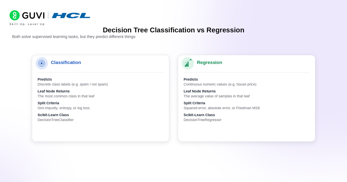
Decision Trees can solve both classification and regression problems, but the target and splitting objective differ.
| Aspect | Classification Tree | Regression Tree |
| Target | Categorical | Continuous |
| Example | Fraud / Legitimate | House Price |
| Output | Class label or probability | Numerical value |
| Common Split Criteria | Gini, Entropy, Log Loss | Squared Error, Absolute Error, Poisson Deviance |
| Leaf Prediction | Majority class / class probabilities | Mean or median depending on criterion |
Scikit-learn currently supports gini, entropy, and log_loss for DecisionTreeClassifier. DecisionTreeRegressor supports criteria including squared_error, absolute_error, and poisson.
Key Features of Decision Trees in Data Science
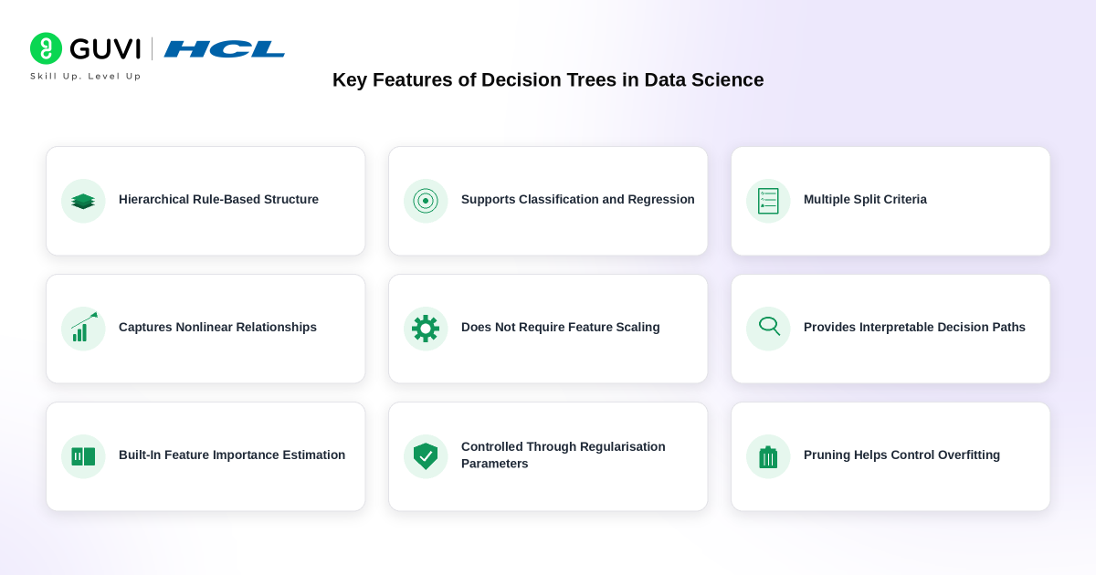
- Hierarchical Rule-Based Structure: A Decision Tree represents predictions as a sequence of conditional rules. The root node contains the complete dataset, internal nodes evaluate feature-based conditions, branches represent the outcome of each condition, and leaf nodes return the final class label or numerical prediction.
- Supports Classification and Regression: Decision Trees can solve both major supervised learning tasks. A
DecisionTreeClassifierpredicts discrete classes, while aDecisionTreeRegressorpredicts continuous values. Classification trees typically optimise impurity measures, while regression trees minimise prediction error within child nodes. - Recursive Feature Splitting: The algorithm repeatedly searches for a feature and threshold that produce the strongest separation of training samples. A numerical feature may create a rule such as
Income <= 50,000, dividing the parent node into child nodes. This recursive partitioning continues until a stopping condition is reached. - Multiple Split Criteria: Classification trees can evaluate candidate splits using measures such as Gini Impurity, Entropy, and Log Loss. Regression trees can use criteria such as squared error, absolute error, Friedman MSE, or Poisson deviance, depending on the implementation. The selected split aims to create child nodes that are more homogeneous than the parent node.
- Captures Nonlinear Relationships and Feature Interactions: Decision Trees do not assume a linear relationship between input variables and the target. Successive splits can model thresholds and interactions automatically. For example, credit risk may depend on income only when debt exceeds a particular threshold.
- Does Not Require Feature Scaling: Tree-based models compare feature values against thresholds rather than calculating distance between observations. Standardisation or normalization is therefore generally unnecessary, unlike algorithms such as KNN, K-Means, or many SVM configurations.
- Provides Interpretable Decision Paths: Every prediction can be traced from the root node to a leaf. This allows developers to inspect which conditions influenced an individual prediction and makes Decision Trees useful when model behaviour needs to be explained.
- Built-In Feature Importance Estimation: Decision Tree implementations can estimate how much each feature contributes to reducing impurity across the tree. In Scikit-learn, this information is available through
feature_importances_. However, impurity-based importance should not be interpreted as causal importance and can favour certain high-cardinality features. - Controlled Through Regularisation Parameters: Tree growth can be restricted using parameters such as
max_depth,min_samples_split,min_samples_leaf,max_leaf_nodes, andccp_alpha. These controls reduce unnecessary branching and help prevent the model from memorising training data. - Pruning Helps Control Overfitting: Fully grown Decision Trees can become deep and highly specific to the training dataset. Pre-pruning limits tree growth during training, while post-pruning, such as cost-complexity pruning, removes branches that provide limited predictive benefit. This can improve generalisation on unseen data.
Build practical machine learning skills and understand how Decision Trees work with HCL GUVI’s Scikit-Learn for Machine Learning Course. Learn model building, classification, regression, Scikit-Learn workflows, and Python-based machine learning through structured hands-on training.
How Decision Trees Choose the Best Split
Choosing the correct split is central to Decision Tree learning.
The exact criterion depends on whether the problem involves classification or regression.
- Gini Impurity
Gini Impurity measures how mixed the classes are inside a node.
It can be represented as:
Gini = 1 – Σpᵢ²
where pᵢ is the proportion of observations belonging to class i.
Suppose a node contains:
- 80 fraud transactions
- 20 legitimate transactions
The probabilities are:
P(Fraud) = 0.8
P(Legitimate) = 0.2
Therefore:
Gini = 1 – (0.8² + 0.2²)
Gini = 0.32
A completely pure node containing only one class has Gini Impurity equal to 0.
The algorithm generally prefers splits that produce lower weighted impurity in the child nodes.
2. Entropy and Information Gain
Entropy also measures uncertainty or disorder inside a node.
The formula is:
Entropy = -Σpᵢ log₂(pᵢ)
A pure node has an entropy of 0.
The Decision Tree calculates how much entropy decreases after a split.
This reduction is called Information Gain:
Information Gain = Parent Entropy – Weighted Child Entropy
A split producing greater Information Gain separates the classes more effectively.
Gini Impurity vs Entropy
Both criteria usually produce similar trees, but they calculate node quality differently.
| Factor | Gini Impurity | Entropy |
| Measures | Class impurity | Information uncertainty |
| Formula | 1 – Σp² | -Σp log₂p |
| Pure Node | 0 | 0 |
| Common Use | CART-style classification | Information Gain-based splitting |
| Computation | Slightly simpler | Uses logarithms |
In practical model development, the difference between the two is often smaller than the effect of parameters such as tree depth and minimum leaf size.
How Regression Trees Select Splits
Regression Trees do not measure class purity because their targets are numerical.
Instead, they attempt to create child nodes containing similar target values.
With squared error, the algorithm searches for splits that reduce variation around the leaf mean.
Suppose a house-price dataset contains:
- Area
- Number of bedrooms
- Location score
- Property age
- Sale price
The tree may split first on:
Area <= 1500 sq. ft.
Each resulting group is then evaluated for another split that further reduces prediction error.
Scikit-learn’s current DecisionTreeRegressor uses squared_error by default.
Key Applications of Decision Trees in Data Science

Decision Trees are especially useful when relationships between features and outcomes can be represented through interpretable rules.
1. Fraud Detection
A fraud model may consider:
- Transaction amount
- Login location
- Transaction frequency
- Device type
- Account age
The resulting tree may identify combinations of features associated with suspicious activity.
2. Customer Churn Prediction
Decision Trees can classify customers as likely or unlikely to churn using:
- Subscription duration
- Monthly spending
- Support requests
- Product usage
- Renewal history
3. Credit Risk Assessment
Financial models may use:
- Income
- Credit score
- Existing debt
- Repayment history
- Loan amount
to estimate whether an applicant belongs to a higher-risk category.
4. Sales and Demand Prediction
Regression Trees can estimate:
- Product demand
- Revenue
- Customer spending
- Inventory requirements
using historical business features.
5. Customer Segmentation Rules
Although Decision Trees are supervised rather than clustering algorithms, they can help translate known customer segments into interpretable classification rules.
6. Operational Risk and Predictive Maintenance
Sensor measurements, equipment age, temperature, pressure, and maintenance history can be used to classify equipment failure risk.
Advantages of Decision Trees in Data Science
Decision Trees offer several practical advantages.
1. Highly Interpretable
A prediction can be traced through explicit conditions.
For example:
Age <= 30 → Income > 40000 → High Purchase Probability
This makes Decision Trees useful when stakeholders need understandable decision logic.
2. Handles Nonlinear Relationships
Decision Trees do not assume a linear relationship between features and the target.
They can model threshold effects and feature interactions naturally.
3. Does Not Require Feature Scaling
Algorithms such as K-Nearest Neighbours and Support Vector Machines can be sensitive to feature scales.
Decision Trees select thresholds on individual features, so standardization or normalization is usually unnecessary.
4. Supports Classification and Regression
The same tree-based framework can solve categorical and continuous prediction problems.
5. Captures Feature Interactions
The effect of one feature can depend on conditions established earlier in the tree.
For example:
If Age < 30, then evaluate Income
but:
If Age >= 30, then evaluate Credit Score
6. Can Provide Feature Importance
Tree models can calculate impurity-based feature importance.
However, this importance should be interpreted carefully because features with many possible split points can receive misleadingly high importance. Permutation importance can provide an alternative assessment.
How Decision Trees Work

A Decision Tree works by recursively partitioning a dataset into smaller and more homogeneous subsets. At each stage, the algorithm selects a feature and split point that best separates the target variable. This process creates a hierarchy of root nodes, internal decision nodes, branches, and leaf nodes.
1. Root Node Starts With the Complete Dataset
The root node is the first node in the tree and contains all training samples.
The algorithm evaluates candidate features and thresholds to determine which split produces the greatest improvement in target separation.
For example, a credit-risk tree may begin with:
Annual Income <= ₹8,00,000?The dataset is then divided into two child groups depending on whether the condition is true or false.
2. The Algorithm Evaluates Candidate Splits
For numerical features, the tree tests different threshold values.
For example:
Age <= 35
Income <= 600000
Credit Score <= 720
For each candidate split, the algorithm measures how much the resulting child nodes improve purity or reduce prediction error.
In classification problems, commonly used criteria include:
- Gini Impurity
- Entropy
- Log Loss
Gini impurity is calculated as:\[ Gini = 1 – \sum_{i=1}^{C} p_i^2 \]
where pᵢ is the proportion of samples belonging to class i.
A node containing mostly one class has lower impurity than a node containing a balanced mixture of classes.
3. The Best Split Becomes an Internal Node
An internal node, also called a decision node, contains a condition that divides samples into child nodes.
For example:
Credit Score <= 650?Samples satisfying the condition follow one branch, while the remaining samples follow another.
In Scikit-learn, Decision Trees typically create binary splits, meaning each internal node produces two child nodes.
4. Branches Represent Split Outcomes
Branches connect one decision node to the next.
For a condition such as:
Age <= 30the branches may represent:
True  -> Left Child
False -> Right Child
As samples move through successive branches, the feature space is divided into increasingly smaller regions.
5. Recursive Partitioning Continues
The algorithm repeats the same process independently for each child node:
Choose Feature
      ↓
Choose Threshold
      ↓
Measure Split Quality
      ↓
Select Best Split
      ↓
Create Child Nodes
      ↓
Repeat
This recursive process allows the tree to capture nonlinear relationships and interactions between features.
For example, loan approval may depend on income only when the applicant’s existing debt is above a particular level. A Decision Tree can represent this interaction naturally through successive splits.
6. Leaf Nodes Produce Final Predictions
A leaf node is a terminal node where no additional split is performed.
For classification, the prediction is typically based on the class distribution of training samples reaching that leaf.
Suppose a leaf contains:
Approved: 42
Rejected: 8
The predicted class would generally be:
ApprovedThe estimated class probability would be approximately:
P(Approved) = 42 / 50 = 0.84For regression, the leaf returns a numerical value derived from the target values of samples in that region, commonly their mean when squared error is used.
7. Tree Growth Stops Based on Defined Conditions
A Decision Tree should not split indefinitely.
Growth may stop when:
- A node reaches the maximum allowed depth.
- Too few samples remain to create another split.
- A leaf reaches the minimum sample requirement.
- No candidate split provides sufficient improvement.
- The maximum number of leaf nodes is reached.
- A pruning rule removes unnecessary branches.
Important Scikit-learn controls include:
max_depth
min_samples_split
min_samples_leaf
max_leaf_nodes
min_impurity_decrease
ccp_alpha
These parameters help control model complexity.
8. Prediction Follows One Root-to-Leaf Path
Once the tree is trained, a new observation passes through only one path.
For example:
Root:
Income <= 700000?
        |
       Yes
        ↓
Credit Score <= 680?
        |
        No
        ↓
Debt Ratio <= 0.35?
        |
       Yes
        ↓
Leaf: Approve Loan
Each prediction can therefore be traced through a sequence of explicit rules.
This makes Decision Trees easier to interpret than many black-box machine learning models.
9. Classification and Regression Trees Use Different Split Objectives
The tree structure is similar for both tasks, but the optimization objective changes.
| Task | Typical Split Criteria | Leaf Output |
|---|---|---|
| Classification | Gini, Entropy, Log Loss | Class or class probability |
| Regression | Squared Error, Friedman MSE, Absolute Error, Poisson | Numerical prediction |
A classification tree tries to create purer class distributions, while a regression tree attempts to reduce the variation of continuous target values within each child node.
10. Pruning Controls Overfitting
A fully grown tree may create highly specific rules that fit noise in the training data.
This causes overfitting.
Two approaches help control it:
- Pre-pruning: Restricts tree growth using parameters such as
max_depth,min_samples_split, ormin_samples_leaf. - Post-pruning: Grows a larger tree and later removes branches that contribute little predictive value.
Scikit-learn supports cost-complexity pruning through ccp_alpha.
The objective is not to create the deepest possible tree, but to find a tree that captures useful patterns while still generalizing to unseen data.
Decision Tree Example: How a Prediction Is Made

- The first condition for a fit person is, they should be below 30 years old.
- The second condition is to check whether the person eats a lot of pizzas or exercises in the morning.
- Based on the two conditions, the decision tree will predict whether the person is fit or unfit.
Example 1:
Suppose a person is 35 years old and exercises in the morning.
The prediction path is:
Age < 30? → No → Exercises in the morning? → Yes → Fit
Because the first condition is false, the observation moves to the right child node. The second condition evaluates exercise behaviour. Since the person exercises in the morning, the sample reaches the Fit leaf node.
Technically, the model does not calculate the prediction using all features simultaneously. It evaluates only the features encountered along that specific root-to-leaf decision path.

Example 2:
Now consider a person who is 28 years old and eats a lot of pizza.
The prediction path becomes:
Age < 30? → Yes → Eats a lot of pizza? → Yes → Unfit

The first split routes the observation to the left subtree because the age condition is satisfied. The second internal node evaluates eating behaviour, after which the sample reaches the Unfit leaf.

Implementing Decision Trees in Data Science: Step-by-Step

Implementing a Decision Tree involves more than fitting a model to a dataset. A reliable workflow includes data preparation, train-test splitting, model configuration, training, prediction, evaluation, interpretation, and hyperparameter tuning.
The following example uses Scikit-learn to build a Decision Tree classification model in Python.
Step 1: Import the Required Libraries
Start by importing the dataset, preprocessing utilities, Decision Tree model, and evaluation metrics.
from sklearn.datasets import load_irisfrom sklearn.model_selection import train_test_splitfrom sklearn.tree import DecisionTreeClassifier, plot_treefrom sklearn.metrics import ( accuracy_score, classification_report, confusion_matrix)import matplotlib.pyplot as pltThe main components are:
train_test_splitseparates training data from unseen test data.DecisionTreeClassifierbuilds the classification tree.plot_treevisualizes learned decision rules.accuracy_scoremeasures overall prediction accuracy.classification_reportprovides precision, recall, and F1-score.confusion_matrixshows how predicted classes compare with actual classes.
Step 2: Load and Inspect the Dataset
For this example, use the Iris dataset.
iris = load_iris()X = iris.datay = iris.targetprint(X.shape)print(iris.feature_names)print(iris.target_names)The dataset contains 150 observations, four numerical input features, and three target classes.
The input features are:
- Sepal length
- Sepal width
- Petal length
- Petal width
The target variable identifies the Iris species.
Before training any Decision Tree, developers should inspect:
- Number of samples
- Feature data types
- Missing values
- Class distribution
- Potential outliers
- Target variable structure
Decision Trees do not require feature standardization because they split observations using thresholds instead of distance calculations.
Step 3: Split the Data Into Training and Test Sets
The model should be trained and evaluated on separate data.
X_train, X_test, y_train, y_test = train_test_split( X, y, test_size=0.20, random_state=42, stratify=y)Here:
test_size=0.20reserves 20% of the data for testing.random_state=42makes the split reproducible.stratify=ypreserves approximately the same class distribution in both subsets.
The model learns decision rules using X_train and y_train. The test set remains unseen until evaluation.
Step 4: Configure the Decision Tree Model
Create the classifier with selected hyperparameters.
model = DecisionTreeClassifier( criterion="gini", max_depth=4, min_samples_split=2, min_samples_leaf=1, random_state=42)Important parameters include:
criterion: Determines how split quality is measured. Common options includegini,entropy, andlog_loss.max_depth: Limits how many levels the tree can grow.min_samples_split: Defines the minimum number of samples required before an internal node can split.min_samples_leaf: Defines the minimum number of samples allowed in a leaf node.max_features: Limits how many features are considered when searching for each split.ccp_alpha: Controls cost-complexity pruning.
Without restrictions, a tree may continue splitting until leaves become extremely specific to the training data, increasing the risk of overfitting.
Step 5: Train the Decision Tree
Fit the model using the training data.
model.fit(X_train, y_train)During training, the algorithm evaluates possible feature thresholds.
For example, it may test conditions such as:
petal width <= 0.8
petal length <= 4.75
sepal length <= 5.9
For every candidate split, the algorithm measures how much the split reduces impurity.
If Gini impurity is used:\[ Gini = 1 – \sum_{i=1}^{C} p_i^2 \]
where pᵢ represents the proportion of samples belonging to class i.
A lower Gini value indicates a purer node.
The algorithm recursively repeats this process until a stopping rule is reached.
Step 6: Generate Predictions
After training, use the model to predict classes for unseen observations.
y_pred = model.predict(X_test)You can also retrieve estimated class probabilities:
y_prob = model.predict_proba(X_test)print(y_prob[:3])For each observation, predict_proba() returns the proportion of training samples from each class contained in the reached leaf.
For example:
[0.00, 0.95, 0.05]indicates that the corresponding leaf strongly favours the second class.
Step 7: Evaluate Model Performance
Accuracy alone may not provide enough information.
accuracy = accuracy_score(y_test, y_pred)print("Accuracy:", accuracy)print(classification_report(y_test, y_pred))print(confusion_matrix(y_test, y_pred))Important classification metrics include:
- Accuracy: Percentage of all predictions that are correct.
- Precision: Percentage of predicted positives that are actually positive.
- Recall: Percentage of actual positives correctly identified.
- F1-Score: Harmonic mean of precision and recall.
- Confusion Matrix: Shows true and false predictions for every class.
For imbalanced datasets, precision, recall, F1-score, ROC-AUC, or PR-AUC may provide more useful information than accuracy alone.
Step 8: Visualize the Decision Tree
One major advantage of Decision Trees is that their learned rules can be inspected visually.
plt.figure(figsize=(16, 8))plot_tree( model, feature_names=iris.feature_names, class_names=iris.target_names, filled=True, rounded=True)plt.show()Each node typically displays information such as:
- Split condition
- Impurity value
- Number of samples
- Class distribution
- Predicted class
A path through the tree can therefore be interpreted as a sequence of decision rules.
For example:
Petal length <= 2.45
        |
       Yes
        |
Predict Setosa
This interpretability is one reason Decision Trees are useful in applications where prediction logic needs to be inspected.
Step 9: Examine Feature Importance
Scikit-learn provides impurity-based feature importance scores.
for feature, importance in zip( iris.feature_names, model.feature_importances_): print(feature, importance)A higher value indicates that the feature contributed more to impurity reduction across the trained tree.
However, these values should be interpreted carefully. Impurity-based importance can favour variables with many possible split points and does not establish causal relationships.
Permutation importance or SHAP-based analysis can provide additional insight when feature interpretation is important.
Step 10: Tune the Decision Tree
A Decision Tree that performs extremely well on training data but poorly on test data is probably overfitting.
Common parameters to tune include:
max_depth
min_samples_split
min_samples_leaf
max_features
max_leaf_nodes
criterion
ccp_alpha
For example:
model = DecisionTreeClassifier( max_depth=5, min_samples_split=10, min_samples_leaf=5, ccp_alpha=0.001, random_state=42)Hyperparameters should ideally be selected using cross-validation rather than repeatedly checking performance on the final test set.
Tools such as GridSearchCV and RandomizedSearchCV can systematically evaluate parameter combinations.
Step 11: Use Decision Trees for Regression
The same basic workflow applies to regression problems.
Instead of:
DecisionTreeClassifieruse:
from sklearn.tree import DecisionTreeRegressorregressor = DecisionTreeRegressor( criterion="squared_error", max_depth=5, random_state=42)regressor.fit(X_train, y_train)DecisionTreeRegressor supports criteria such as:
squared_errorfriedman_mseabsolute_errorpoisson
Instead of predicting classes, regression trees place observations into regions and return numerical predictions based on the target values of training samples within each leaf.
Complete Decision Tree Workflow
A practical Decision Tree pipeline can therefore be summarized as:
Collect Data → Inspect Features → Split Dataset → Configure Tree → Train Model → Predict → Evaluate → Visualize → Tune Hyperparameters → Validate on Unseen Data
Following this workflow helps ensure that the Decision Tree is not only accurate on training data but also interpretable, controlled for overfitting, and suitable for real-world prediction tasks.
Decision Tree vs Random Forest vs Gradient Boosting
A single Decision Tree prioritizes interpretability, while ensemble methods combine multiple trees to improve predictive performance.
| Factor | Decision Tree | Random Forest | Gradient Boosting |
| Number of Trees | One | Many | Many sequential trees |
| Interpretability | High | Moderate to low | Low |
| Overfitting Risk | High if unrestricted | Lower than one tree | Controlled through tuning |
| Training Method | Recursive splitting | Bagging + random feature subsets | Sequential error correction |
| Prediction Power | Good baseline | Usually stronger | Often very strong |
| Parallel Training | Single model | Highly parallelizable | More sequential |
| Best Use | Explainable baseline | Robust general-purpose prediction | High-performance tabular modelling |
A Decision Tree is often the best place to learn tree-based modelling because Random Forest and boosting methods build on the same fundamental idea of recursive partitioning.
Common Mistakes When Building Decision Trees
1. Training and Testing on the Same Dataset
Evaluating a model on its training data produces an unrealistically optimistic estimate.
Always preserve unseen validation or test data.
2. Allowing Unlimited Tree Growth
An unrestricted tree can memorize individual training observations.
Control complexity using depth, leaf-size, impurity, or pruning parameters.
3. Evaluating Only Accuracy
For imbalanced classification, a model can achieve high accuracy by repeatedly predicting the majority class.
Also examine:
- Precision
- Recall
- F1-score
- Confusion matrix
- ROC-AUC or PR-AUC where appropriate
4. Treating Feature Importance as Causality
A high importance score means a feature contributed strongly to the tree’s splits.
It does not prove that changing the feature would cause the target outcome to change.
5. Ignoring Class Imbalance
For highly imbalanced targets, consider:
DecisionTreeClassifier(
class_weight=”balanced”
)
Scikit-learn can automatically assign class weights inversely related to class frequencies when class_weight=”balanced” is used.
6. Using a Very Small Toy Dataset as Proof of Performance
A model trained on six or ten manually created observations cannot demonstrate realistic predictive performance.
Use sufficiently representative datasets and proper validation.
How to Improve Decision Tree Performance
A stronger Decision Tree workflow usually includes:
- Clean and validate the dataset.
- Separate training, validation, and test data where appropriate.
- Establish an unrestricted or lightly constrained baseline.
- Inspect tree depth and leaf counts.
- Tune max_depth.
- Tune min_samples_split.
- Tune min_samples_leaf.
- Evaluate cost-complexity pruning.
- Use cross-validation.
- Compare against ensemble baselines.
The objective is not to build the deepest possible tree.
It is to find the smallest tree that generalizes well enough for the problem.
When Should You Use a Decision Tree?
Decision Trees are particularly useful when:
- Interpretability is important.
- Feature interactions are expected.
- Relationships are nonlinear.
- Data is primarily tabular.
- A transparent baseline model is required.
- Feature scaling should be avoided.
- Business rules need to be extracted from model behaviour.
A different model may be preferable when:
- Very high predictive accuracy is more important than interpretability.
- Small data changes make the tree unstable.
- Raw images, audio, or text embeddings dominate the input.
- Smooth extrapolation is required.
- The relationship is better captured by another model family.
Decision Trees in Modern Data Science
Decision Trees remain highly relevant because tree-based models dominate many structured and tabular machine learning problems.
Their importance extends beyond standalone Decision Trees.
The same recursive splitting concept appears in:
- Random Forest
- Extra Trees
- AdaBoost
- Gradient Boosting
- XGBoost
- LightGBM
- CatBoost
Learning how a single tree chooses splits, creates leaves, overfits, and gets pruned makes these more advanced algorithms easier to understand.
Limitations of Decision Trees
Decision Trees in machine learning are simple to understand but can develop several modelling problems.
1. Overfitting
An unrestricted tree may continue splitting until it captures noise and individual training examples.
This produces excellent training performance but weak generalization.
2. Model Instability
Small changes in the training dataset can produce different split points and a significantly different tree.
3. Greedy Split Selection
A Decision Tree chooses the best split available at the current node.
It does not search every possible future tree structure for a globally optimal solution.
4. Poor Extrapolation in Regression
Regression Trees create piecewise constant predictions.
They generally cannot extrapolate smoothly beyond patterns represented in the training data.
5. Deep Trees Lose Interpretability
A tree with three levels may be easy to explain.
A tree containing hundreds of nodes is technically interpretable but difficult for a human to understand.
6. Impurity-Based Feature Importance Can Mislead
Features with many unique values may appear artificially important.
Feature importance should therefore be validated using techniques such as permutation importance or SHAP when interpretation matters.
Conclusion
Decision Trees provide one of the clearest ways to understand how supervised machine learning converts features into predictions. They recursively divide data using criteria such as Gini Impurity, Entropy, or regression error until observations reach terminal leaves containing the final output.
Their interpretability makes them valuable for explainable tabular modelling, but unrestricted trees can overfit and become unstable. Parameters such as max_depth, min_samples_split, min_samples_leaf, and ccp_alpha help control complexity and improve generalization.
Understanding Decision Trees also creates a strong foundation for Random Forest, Gradient Boosting, and other advanced tree-based models widely used across modern Data Science.
FAQs
Q1. Do I need coding for data science?
Yes, coding is an essential skill for data science. Being comfortable with coding is crucial for tasks like data manipulation, building machine learning models, and automating processes. Python and R are the most commonly used programming languages in data science, and they have extensive libraries to make your job easier.
Q2. Is DSA required for data science?
Yes, Data Structures and Algorithms (DSA) are important for data science, especially for machine learning and data engineering. DSA helps with data management, analysis, and problem solving. It can also help you write efficient code. You can expect DSA-based coding challenges during the interview.
Q3. Which language is best for data science?
The most popular and widely used language for data science is Python. It’s beginner-friendly, has a rich ecosystem of libraries (like Pandas, NumPy), and is great for tasks like data cleaning, analysis, and machine learning. For those working on large-scale systems, Scala and Julia are gaining popularity as well, especially for machine learning and high-performance tasks.
Q4. What industries hire data scientists?
Data scientists are in demand everywhere, from tech giants like Google and Amazon to healthcare, finance, retail, and entertainment. Almost every industry is tapping into data to drive smarter decisions.
Q5. Is data science a good career for freshers
Absolutely! With the booming demand for data-driven insights, freshers with strong analytical skills and a passion for learning can easily find opportunities and grow rapidly in the field.
Success Stories

About the Author
Vaishali
I'm a seasoned writer with four years of experience across technical, non-technical, and just about every genre or niche you can imagine. Adaptable and curious, I enjoy exploring new topics and making information engaging and easy to understand. Fueled by a steady stream of tea, I approach each project with creativity, reliability, and genuine enthusiasm for storytelling.
View all posts by Vaishali
Connect with me @










Did you enjoy this article?