Linear Regression in Data Science: A Beginner’s Guide

Ever wondered how Netflix predicts your next favorite show or how Amazon remembers your preferences and suggests according to them? Behind the scenes, there’s a simple yet powerful algorithm at work: linear regression. 

It’s one of the first tools data scientists reach for when trying to understand relationships between variables or forecast future trends. Linear regression in data science is a foundational technique in machine learning for modeling and predicting continuous outcomes.

In this article, you’ll explore how simple and multiple linear regression work, the key assumptions behind the model, how we evaluate its performance, how to implement it in Python, and where it’s used in real-world problems. So, without further ado, let us get started!

Simple vs. Multiple Linear Regression in Data Science

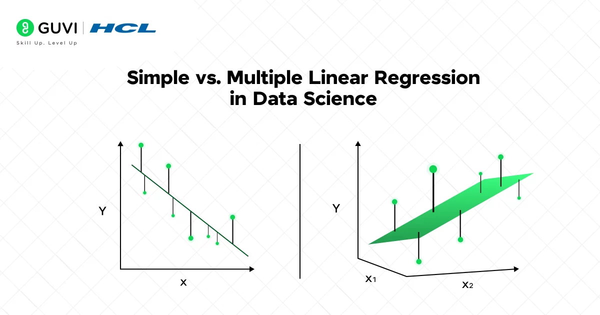
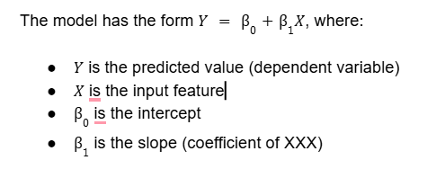
The distinction between simple and multiple linear regression in data science is straightforward. In simple linear regression, you model the relationship between a single input (independent) variable X and one output (dependent) variable Y. 

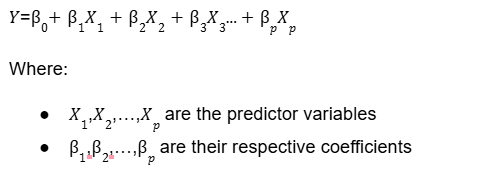
In multiple linear regression, there are two or more input features. The model becomes 

In practice, linear regression “predicts relationships between variables by fitting a line that minimizes prediction errors”. 

For example, a simple model might predict a student’s exam score from hours studied, while a multiple regression might use hours studied, attendance, and previous grades together. In both cases, the model finds coefficients (slopes) that best explain the observed data.

Model Specification

When you fit a linear model, you are estimating the coefficients that minimize the sum of squared errors between the predicted and actual values. In simple linear regression, this is just fitting a line through scatter-plot data.

With multiple features, imagine a hyperplane in higher dimensions that best fits all points. This fitting process assumes a linear relationship between each feature and the target, though the overall model can use many features at once.

Assumptions of Linear Regression

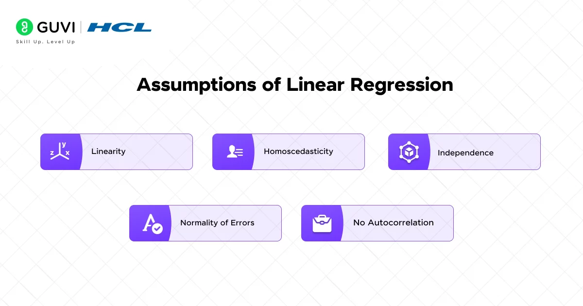
Linear regression relies on several key assumptions for its results to be valid. Understanding these assumptions helps you decide when linear regression is appropriate and how to diagnose issues. As a rule of thumb, these include linearity, independence, homoscedasticity, and normality of errors, among others:

• Linearity: The relationship between each predictor and the target must be linear. You can check this by plotting each feature against the target – the pattern should look roughly like a straight line. If the true relationship is highly non-linear (e.g., exponential), a plain linear model will perform poorly.
  
• Homoscedasticity: The residuals (prediction errors) should have constant variance across all levels of the inputs. In other words, the “spread” of errors should look uniform in a residual plot. If errors fan out (widen) or narrow as X increases, this heteroscedasticity can violate assumptions and affect confidence in predictions.
  
• Independence: The observations should be independent of each other. In time-series data or grouped data, autocorrelation or clustering can violate this. Also, the features should not be perfectly collinear (no multicollinearity) – that is, no two predictors should be linearly redundant.
  
• Normality of Errors: The residuals should be normally distributed (around zero mean). This mainly affects confidence intervals and hypothesis testing; the estimators for coefficients are still unbiased without normality, but inference (p-values, confidence intervals) assumes it.
  
• No Autocorrelation: Especially in time-dependent data, successive residuals should not be correlated; this is the “independence” assumption applied to errors. Tools like the Durbin-Watson test can check this.
  

In practice, you should always check these assumptions when using linear regression. Scatter plots, residual plots, Q-Q plots, and variance inflation factors (VIF) are common diagnostics. Violations don’t always “break” the model, but they do affect how much you can trust standard errors and p-values, and indicate whether transformations or different models might be needed. 

Model Evaluation Metrics

Once you fit a linear regression model, you need to evaluate how well it performs. Two of the most common metrics are the coefficient of determination (R²) and the Root Mean Squared Error (RMSE).

R-squared (R²): This metric indicates the proportion of the variance in the target that is explained by the model. It ranges from 0 to 1 (higher is better) – an R² of 1.0 means the model perfectly fits the data, while 0 means it explains none of the variance. (On new or test data, R² can be negative if the model fits worse than a horizontal line at the mean.)

In practice, you might compute it using r2_score in scikit-learn. R2 is useful to quickly gauge model quality, but it has limits – for example, it doesn’t tell you anything about bias vs. variance or absolute prediction error.

Root Mean Squared Error (RMSE): This is the square root of the average squared difference between predicted and actual values.

RMSE is on the same scale as the target variable, making it intuitive: it tells you roughly how far off your predictions are, on average. A smaller RMSE means better predictive accuracy. Because it squares errors, it penalizes larger errors more heavily.

Both metrics are widely used. For example, after predicting with a linear model in scikit-learn, you could do:

python

from sklearn.metrics import r2_score, mean_squared_error

r2 = r2_score(y_test, y_pred)

rmse = np.sqrt(mean_squared_error(y_test, y_pred))

R² (via r2_score) will give you the coefficient of determination, and RMSE (via mean_squared_error) gives the error magnitude. In practice, you might also look at Mean Absolute Error (MAE) or Adjusted R² (which penalizes having too many features), depending on the context.

Monitoring these metrics is important. A very high R² on training data (e.g. 0.98) might look good, but you should always check performance on a validation or test set. A model with R²=0.95 on training and 0.50 on test probably isn’t generalizing well (likely overfitting). 

In general, R² tells you the relative quality of fit (variance explained), while RMSE tells you the absolute error scale.

Interactive Challenge: 

Suppose you fit a linear regression on training data and achieve R² = 0.90. On new test data, however, R² drops to 0.50. What might this suggest about your model? Think about overfitting, underfitting, or data leakage, and what steps (like adding data, simplifying the model, or cross-validation) you might take to improve the situation.

Implementing Linear Regression (scikit-learn)

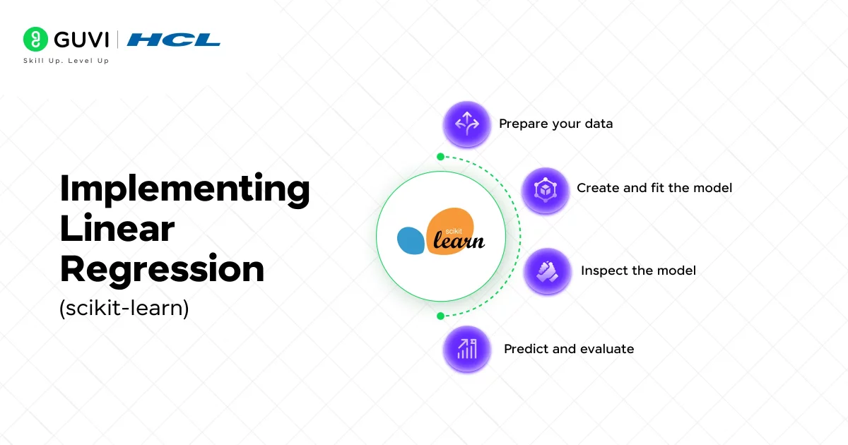
In Python, you can build linear regression models easily with libraries like scikit-learn. The LinearRegression class in sklearn.linear_model implements ordinary least squares. A typical workflow is:

1. Prepare your data: Split into features X and target y, and into training/testing sets (e.g., using train_test_split).
   
2. Create and fit the model:
   
   from sklearn.linear_model import LinearRegression
model = LinearRegression()
model.fit(X_train, y_train)

This will learn the coefficients that best fit the training data.

3. Inspect the model: After fitting, model.coef_ gives the slope(s) for each feature, and model.intercept_ gives the y-intercept (bias). For example, if X has one column, model.coef_[0] is the slope of the line, and model.intercept_ is the intercept.
   
4. Predict and evaluate: Use y_pred = model.predict(X_test) to get predictions on new data. Then compute metrics: r2_score(y_test, y_pred), mean_squared_error(y_test, y_pred), etc., as shown above.

Using scikit-learn abstracts away the math of solving normal equations (or gradient descent). Under the hood, LinearRegression solves for the coefficients. Because linear regression has no hyperparameters (except fit_intercept=True by default), you typically only need to worry about data preprocessing. 

Besides scikit-learn, many people also use statsmodels in Python for linear regression, which provides more statistical output (like p-values, confidence intervals). But for straightforward predictive modeling, scikit-learn’s LinearRegression is usually sufficient.

If you want to read more about how much linear regression is important in Data Science, consider reading GUVI’s Free Ebook: Master the Art of Data Science – A Complete Guide, which covers the key concepts of Data Science, including foundational concepts like statistics, probability, and linear algebra, along with essential tools.

Real-World Use Cases of Linear Regression in Data Science

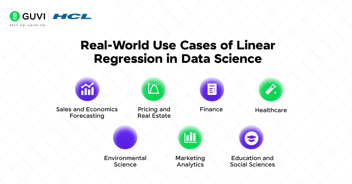
Linear regression is ubiquitous in data-driven fields because many problems start with asking “is there a linear trend?” or “Can we predict this outcome as a weighted sum of factors?”. Here are some typical use cases:

• Sales and Economics Forecasting: You might use linear regression to forecast how many items a store will sell based on factors like past sales, advertising spend, seasonality, or even weather. For example, a retailer could predict next month’s sales from historical sales and marketing budgets. In economics, analysts often regress GDP growth on indicators like interest rates, exports, and consumption to understand trends.
  
• Pricing and Real Estate: A classic example is predicting house prices. By regressing sale price against features like square footage, location, number of bedrooms, etc., one can estimate property values. Similarly, companies predict product prices or demand based on cost factors and market variables.
  
• Finance: Linear regression can estimate relationships in finance, such as predicting stock returns from economic indicators or finding the beta of a stock via regression.
  
• Healthcare: Doctors and researchers use linear regression to model outcomes like blood pressure or risk scores as a function of age, weight, lifestyle factors, and treatment dosages. For example, predicting patient blood sugar from diet and exercise data is a regression task.
  
• Environmental Science: Scientists might predict pollution levels or climate variables based on factors like emissions data, temperature, and human activity.
  
• Marketing Analytics: Linear models can quantify the effect of advertising spend on sales, or how customer demographics relate to purchase amounts.
  
• Education and Social Sciences: Educators might predict test scores from study hours and attendance. Social scientists often regress outcomes (income, vote share, etc.) on demographic and historical data.

In general, if you have data that seems roughly linear and you want an easy-to-interpret model, linear regression is a good starting point. Its coefficients directly tell you how changing an input moves the output, which is great for interpretability.

If you want to learn more about how Linear Regression is crucial for data science through a structured program that starts from scratch, consider enrolling in GUVI’s IIT-M Pravartak Certified Data Science Course, which empowers you with the skills and guidance for a successful and rewarding data science career 

Conclusion

In conclusion, linear regression remains a fundamental tool in data science. It’s often your “first attempt” for any continuous prediction problem because of its simplicity, speed, and interpretability. 

As you move forward, remember that linear regression is both a practical modeling technique and a stepping stone to more complex methods. It’s an invaluable starting point in any data science project. 

Keep building on this foundation – linear regression will pop up often, and understanding it thoroughly will serve you well in more advanced modeling tasks.

FAQs