
What is Classification in Data Science? A Simple Guide
Oct 08, 2025 6 Min Read 2702 Views
(Last Updated)
Have you ever wondered how your email automatically filters out spam amidst the overflowing emails? That’s the magic of classification in data science.
Classification is one of the most widely used techniques in data science, particularly in machine learning, enabling computers to categorize data into distinct groups. No matter the need, whether it’s determining if an email is spam, diagnosing a disease, or recognizing faces in photos, classification helps make sense of the complex world around us.
But how does it work? Let’s break it down. In this article, we’ll explore what classification in data science is, the different types of classification problems, common algorithms, how to evaluate classification models, and typical use cases.
Table of contents
- What is Classification in Data Science?
- Types of Classification Problems
- Common Classification Algorithms in Data Science
- Logistic Regression
- Decision Trees
- Random Forest (Ensemble of Trees)
- Support Vector Machines (SVM)
- k-Nearest Neighbors (KNN)
- Evaluating Classification Models
- Conceptual Challenge: Put Theory into Practice:
- Real-World Use Cases of Classification in Data Science
- Conclusion
- FAQs
- What is classification in data science?
- What’s the difference between binary and multi-class classification?
- Which algorithms are commonly used for classification?
- How do you evaluate a classification model’s performance?
- What challenges can arise when using classification models?
What is Classification in Data Science?
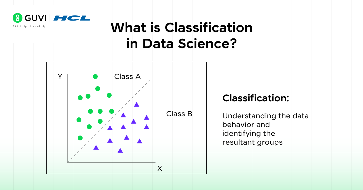
Classification is a fundamental concept in data science and machine learning. In simple terms, classification involves assigning input data to one of several predefined categories or classes.
In supervised learning, a classification model learns from labeled examples and then predicts the class of new, unseen data. For example, a model might learn to label emails as “spam” or “not spam” based on past data.
In other words, a classification model sorts data points into predefined groups called classes. Think of it like a mail sorter that learns to put each piece of mail into the right mailbox (spam or inbox, say) based on its features.
Types of Classification Problems
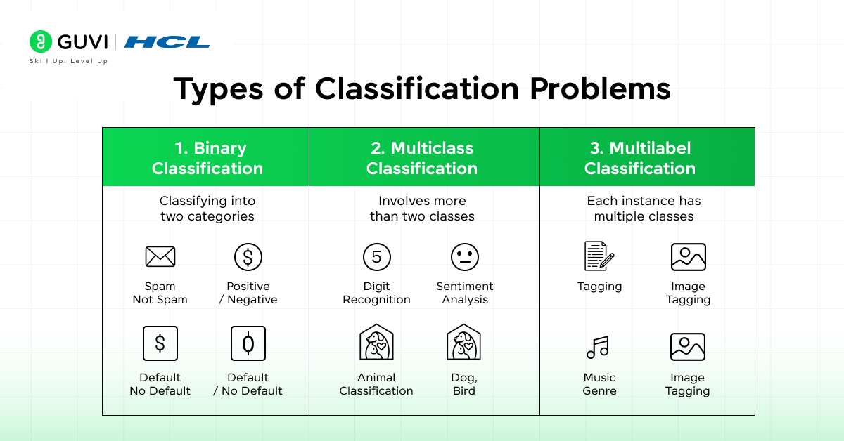
Before diving into algorithms, it’s helpful to understand the different kinds of classification tasks you might encounter:
- Binary Classification: This is the simplest case, where each input is assigned to one of two classes. For example, predicting whether an email is spam or not spam, or whether a patient has a disease (yes/no). In binary classification, the data is labeled in a binary way (e.g., 0/1, true/false, positive/negative).
- Multi-Class Classification: Here, there are more than two possible classes, but still exactly one label per example. For example, an image classifier might label photos as cat, dog, or rabbit. The model must pick one class out of many.
- Multi-Label Classification: In some tasks, each instance can belong to multiple classes simultaneously. For example, a photo might contain both a “bicycle” and an “apple,” so it has two labels. In multi-label classification, a model predicts a set of classes for each example. This is different from multi-class, since examples are not exclusive to one class.
- Imbalanced Classification: Many real-world datasets are imbalanced, meaning some classes have many more examples than others. Examples include fraud detection or rare disease diagnosis.
Common Classification Algorithms in Data Science
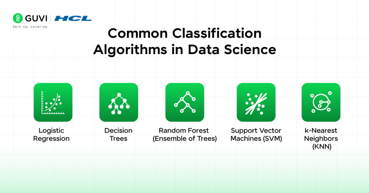
There are many algorithms for classification, each with its strengths and weaknesses. Here are some key ones that you will encounter often:
1. Logistic Regression
Despite its name, logistic regression is used for classification (usually binary). It works by taking a linear combination of input features and applying the sigmoid function to produce a probability between 0 and 1 for one class.
In practice, if the probability is above a threshold (e.g., 0.5), the model predicts class 1; otherwise, class 0. Logistic regression “predicts the probability that an input belongs to a specific class,” making it ideal for problems like yes/no decisions.
It is conceptually simple and interpretable – you can inspect the weights on features. For example, logistic regression has been used to predict the probability of a patient having a disease or for fraud detection.
2. Decision Trees
A decision tree makes decisions by asking a series of yes/no questions about the features, splitting the data into smaller and smaller groups. The result is a tree-like flowchart of decisions, where each leaf node assigns a class.
For example, the root might ask “Is the patient’s temperature > 100°F?” and branch into two nodes, and so on. Decision trees are very intuitive: “flowchart-like” and easy to visualize, so they are transparent and simple for users to understand.
This means you can trace how a decision is made (what questions lead to a certain prediction). Trees work for both classification and regression, and they handle both numerical and categorical data.
3. Random Forest (Ensemble of Trees)
A random forest builds on decision trees by creating a whole “forest” of them. Each tree is trained on a random subset of the data (and features), and then all the trees vote on the final class.
The idea is like consulting many experts rather than relying on one. The forest’s final output is the most common class among the trees. This collective approach usually improves accuracy and reduces overfitting compared to a single tree.
Random forests often achieve high performance because the randomness and averaging make them robust. They can handle a lot of input features and can capture complex interactions. However, they are less interpretable as a whole (though each tree is), and can be slower to train and predict if many trees are used.
4. Support Vector Machines (SVM)
A support vector machine finds the boundary (hyperplane) that best separates the classes in feature space. Imagine plotting data points (with two features, say) and drawing a line that maximally separates the two classes.
SVM searches for the “optimal hyperplane” that has the widest margin (distance) from the nearest points of any class. Points that lie on the margin boundaries are called “support vectors.”
SVMs are powerful and can handle nonlinear boundaries by implicitly mapping data into higher dimensions. For example, an SVM might draw a curved boundary when a simple line won’t do. However, SVMs can be less intuitive than decision trees, and they typically require careful tuning of parameters and kernels.
5. k-Nearest Neighbors (KNN)
KNN is a very simple, intuitive method. To classify a new point, it looks at the k closest training points in the feature space and takes a vote on their classes. In other words, it groups nearby examples and assumes similar points share the same class.
For example, if k=5 and among the 5 nearest neighbors, 3 are labeled “cat” and 2 “dog,” the new point is classified as “cat.” KNN doesn’t build a model ahead of time (it’s a lazy learner); it simply memorizes the training data. At prediction time, it does the computation. This means KNN can be slow on large datasets, but it is very easy to understand and implement.
Each algorithm has its assumptions and strengths. Often, practitioners will try several algorithms and compare them.
Evaluating Classification Models
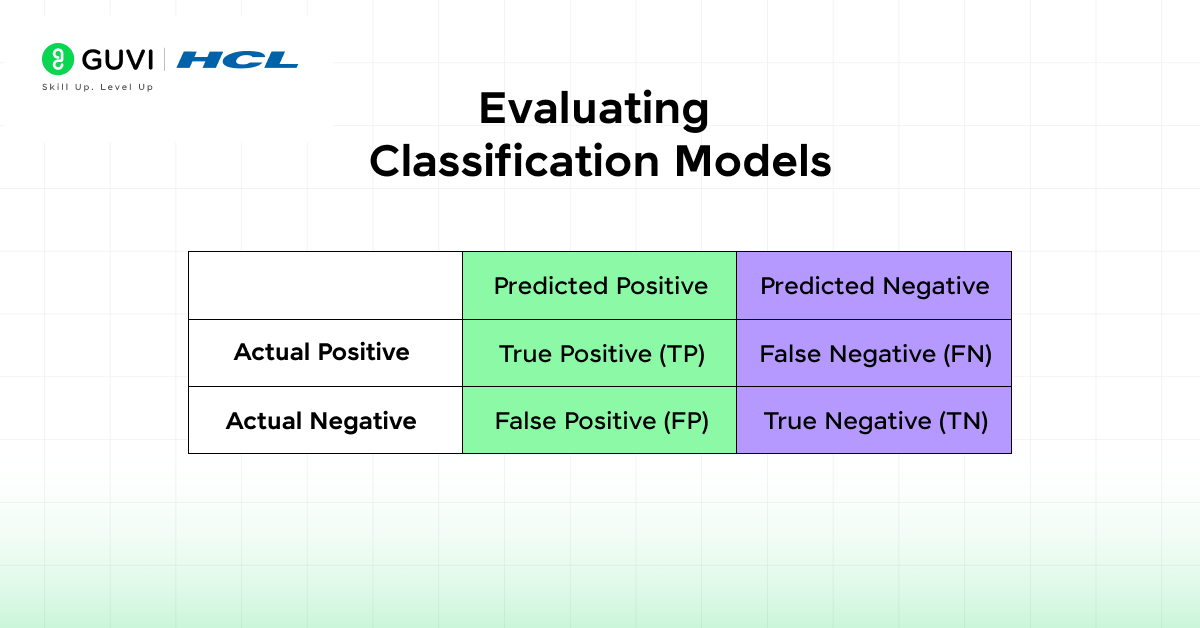
After training a model, you need to evaluate how well it performs. A key tool is the confusion matrix, which tabulates the model’s predictions versus the true labels. For a binary classifier, it looks like this:
| Predicted Positive | Predicted Negative | |
| Actual Positive | True Positive (TP) | False Negative (FN) |
| Actual Negative | False Positive (FP) | True Negative (TN) |
- True Positives (TP): correctly predicted positives.
- False Positives (FP): negative instances incorrectly labeled positive.
- False Negatives (FN): positive instances incorrectly labeled negative.
- True Negatives (TN): correctly predicted negatives.
A confusion matrix “summarizes the performance of a classifier and allows us to identify details that accuracy does not tell us”. From these counts, we compute metrics:
- Accuracy: (TP + TN) / (Total). This tells us the fraction of all correct predictions. It’s a simple overall measure: an accuracy of 0.9 means 90% of predictions matched the true labels. However, accuracy can be misleading, especially with imbalanced data. For example, if 95% of emails are non-spam, a model that always predicts “non-spam” would be 95% accurate but useless.
- Precision: TP / (TP + FP). This measures the quality of positive predictions: out of all instances the model predicted as positive (e.g., “spam”), what fraction were positive. In a spam filter, precision answers: “Of all emails marked spam, how many truly were spam?. High precision means when the model says “yes,” it’s usually correct. Precision is important when false positives are costly.
- Recall (Sensitivity): TP / (TP + FN). This measures coverage of actual positives: out of all true positive cases, what fraction the model identified. In a disease test, recall answers: “Of all the patients who truly have the disease, how many did we catch?” High recall means the model finds most positive cases.
- F1 Score: The harmonic mean of precision and recall. It balances precision vs recall. If you need a single number that considers both, use F1.
Choosing between these metrics depends on the problem. For example, precision vs recall trade-off: In medical diagnosis, you usually prefer recall over precision, because missing a sick patient (false negative) could be life-threatening. In contrast, in spam detection, you might prefer precision to avoid mislabeling important emails as spam.
Conceptual Challenge: Put Theory into Practice:
Suppose you are developing a machine learning model to detect a rare disease (the positive class is rare). Would you prioritize precision or recall? Why? Think about the consequences of each type of error.
(Hint: missing a sick patient (false negative) is much worse than falsely flagging a healthy person as sick in this case.)
Consider your answer: In disease screening, we usually aim for high recall (catch as many actual cases as possible), even if it means some healthy people get flagged incorrectly (lower precision). Missing a real case (false negative) could be disastrous. Conversely, in a spam filter example, you might aim for high precision to avoid incorrectly marking important emails as spam. Optimizing for precision vs recall depends on the real-world costs of false positives and negatives.
If you want to read more about how Classification in Data Science is critical for modelling, consider reading HCL GUVI’s Free Ebook: Master the Art of Data Science – A Complete Guide, which covers the key concepts of Data Science, including foundational concepts like statistics, probability, and linear algebra, along with essential tools.
Real-World Use Cases of Classification in Data Science
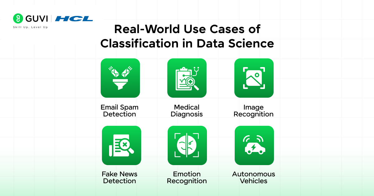
Classification is everywhere in data science applications. Here are some common examples:
- Email Spam Detection: Classify incoming emails as “spam” or “not spam.” A spam filter is a classic binary classification task, using features like email content or sender.
- Medical Diagnosis: Predict whether a patient has a condition (e.g. diabetes, cancer) based on lab tests and symptoms.
- Image Recognition: Classify objects in images. For example, determine if a photo contains a cat, dog, or car. Convolutional neural networks excel at these tasks.
Emerging use cases of classification in data science:
- Fake News Detection: With the rise of misinformation, classifiers are being trained to identify fake news.
- Emotion Recognition: Classification models now detect human emotions from voice, text, and facial expressions.
- Autonomous Vehicles: In self-driving cars, image classifiers identify pedestrians, traffic signs, lane markings, and obstacles in real-time to aid safe navigation.
In short, classification is a powerful and widely used technique in data science. By understanding the types of classification tasks, knowing the algorithms available, and carefully evaluating your models, you can apply classification to solve many real-world problems.
If you want to learn more about how Classification in Data Science is crucial in today’s world and learn everything about it through a structured course taught by actual mentors, consider enrolling in HCL GUVI’s IIT-M Pravartak Certified Data Science Course that empowers you with the skills and guidance for a successful and rewarding data science career
Conclusion
In conclusion, classification in data science enables machines to make smart, structured decisions. From identifying spam emails to diagnosing diseases, its applications are vast and impactful. As a student stepping into this exciting field, understanding how classification works and when to use which algorithm can give you a major head start.
Remember, it’s not just about building a model; it’s about choosing the right one, interpreting the results thoughtfully, and always keeping real-world consequences in mind. With practice and curiosity, you’ll soon be building classifiers that don’t just work, but work smart.
FAQs
1. What is classification in data science?
Classification is a supervised learning technique where a model is trained on labeled data to assign new, unseen instances to predefined categories. It is widely used for tasks like spam detection, image recognition, and medical diagnosis. Essentially, you teach the model to sort inputs into the right “bin.”
2. What’s the difference between binary and multi-class classification?
Binary classification deals with two classes (e.g., spam vs. not spam), while multi-class classification involves more than two (e.g., classifying emails into work, personal, or promotions). The core concept is the same, but multi-class requires the model to handle multiple categories simultaneously.
3. Which algorithms are commonly used for classification?
Popular classification algorithms include logistic regression, decision trees, random forests, support vector machines, k‑nearest neighbors, and Naïve Bayes. Each has its own strengths: trees offer interpretability, while ensembles and SVMs often yield higher accuracy. Your choice depends on data type, interpretability needs, and performance goals.
4. How do you evaluate a classification model’s performance?
Performance is typically measured using metrics like accuracy, precision, recall, and F1‑score derived from the confusion matrix. Accuracy gives overall correctness, precision focuses on correct positive predictions, recall on finding actual positives, and F1 balances both precision and recall.
5. What challenges can arise when using classification models?
Common challenges include class imbalance (e.g., fraud detection), which can mislead accuracy, and overfitting, where a model learns training data too well and performs poorly on new data. Address these with resampling techniques, regularization, or ensemble methods to improve generalization.





Did you enjoy this article?