Beam Search in NLP: How AI Chooses the Best Words 

Every time an AI generates a sentence, whether translating a document, summarising an article, or completing a prompt, it faces a combinatorial explosion. Vocabulary sizes of 30,000 to 50,000 tokens mean that even a 10-word output has an astronomically large space of possible sequences to consider.

Beam Search is the algorithm that makes this tractable. Instead of evaluating every possible sequence or blindly committing to the single best token at each step, it explores multiple promising paths simultaneously, keeping only the top candidates and discarding the rest. The result is outputs that are significantly better than greedy search at a fraction of the cost of exhaustive search.

In this article, we break down exactly how Beam Search works, how it compares to greedy search and exhaustive search, what beam width means in practice, and where this algorithm drives real-world NLP systems today.

TL;DR

•   Beam Search keeps the top-k candidate sequences (beam width = k) at each decoding step.

•        It outperforms greedy search by avoiding locally optimal but globally poor choices.

•      It is far cheaper than exhaustive search, which is computationally infeasible for real sequences.

•        Beam width is the central trade-off: wider beams find better sequences but cost more compute.

•    Beam Search powers machine translation, text summarisation, speech recognition, and caption generation.

The Sequence Generation Problem: Why Decoding Is Hard

Before understanding Beam Search, it helps to understand the problem it solves. Language model decoding, the process of generating an output sequence from a model, is fundamentally a search problem. At every step, the model assigns a probability to every token in its vocabulary. The task is to find the sequence of tokens with the highest overall probability.

The Scale of the Problem

A typical language model vocabulary contains 30,000 to 50,000 tokens. Generating a sequence of length T means searching through V^T possible sequences, where V is the vocabulary size, and T is the sequence length. For a modest 20-token sentence with a 30,000-token vocabulary, that is 30,000^20 candidate sequences, a number far beyond any feasible computation.

• Exhaustive search: Finds the globally optimal sequence but requires evaluating every possible output, computationally infeasible for any real-world vocabulary and sequence length.
• Greedy search: At each step, select the single highest-probability token. Fast and cheap, but makes locally optimal choices that frequently lead to globally suboptimal sequences.
• Beam Search: Maintains the top-k candidates at each step. Significantly better than greedy search, computationally feasible, unlike exhaustive search, it is the practical middle ground.

Greedy Search vs. Beam Search: Understanding the Core Difference

Greedy search is the simplest decoding strategy. At each time step, it selects the token with the highest probability according to the model, appends it to the sequence, and moves on. There is no backtracking, no exploration of alternatives. Once a token is chosen, the decision is final.

 Why Greedy Search Fails

Greedy search fails because the locally optimal choice at step t is not always the globally optimal choice. A token with a slightly lower probability at step t might open up a sequence of highly probable tokens at steps t+1, t+2, t+3, producing a much better overall sequence. Greedy search never discovers this because it commits irreversibly at each step.

A classic example in machine translation: greedy search might select “The bank of the river” when the correct and more natural translation is “The riverbank” because ‘bank’ had the highest single-step probability, but ‘river’ followed by ‘bank’ as a compound noun was globally better. Beam Search, by maintaining multiple hypotheses, can recover from such locally greedy mistakes.

How Beam Search Improves on Greedy

• Instead of committing to one token per step, Beam Search keeps the top-k sequences in the beam.
• At each step, every surviving sequence is extended with every possible next token.
• The resulting k × V candidate sequences are scored by their cumulative log-probability.
• Only the top-k candidates are retained; the rest are pruned.
• The process repeats until all beams produce an end-of-sequence token or a maximum length is reached.

How Beam Search Works: A Step-by-Step Walkthrough

To make Beam Search concrete, let us walk through the algorithm with a small example. This walkthrough demonstrates exactly how the beam evolves at each decoding step and why maintaining multiple hypotheses leads to better final sequences.

Setup

•        Beam width k = 2 (we keep the top 2 sequences at each step).

•        Vocabulary = {The, A, cat, dog, sat, ran, quickly, .}

•        The model outputs a probability distribution over the vocabulary at each step.

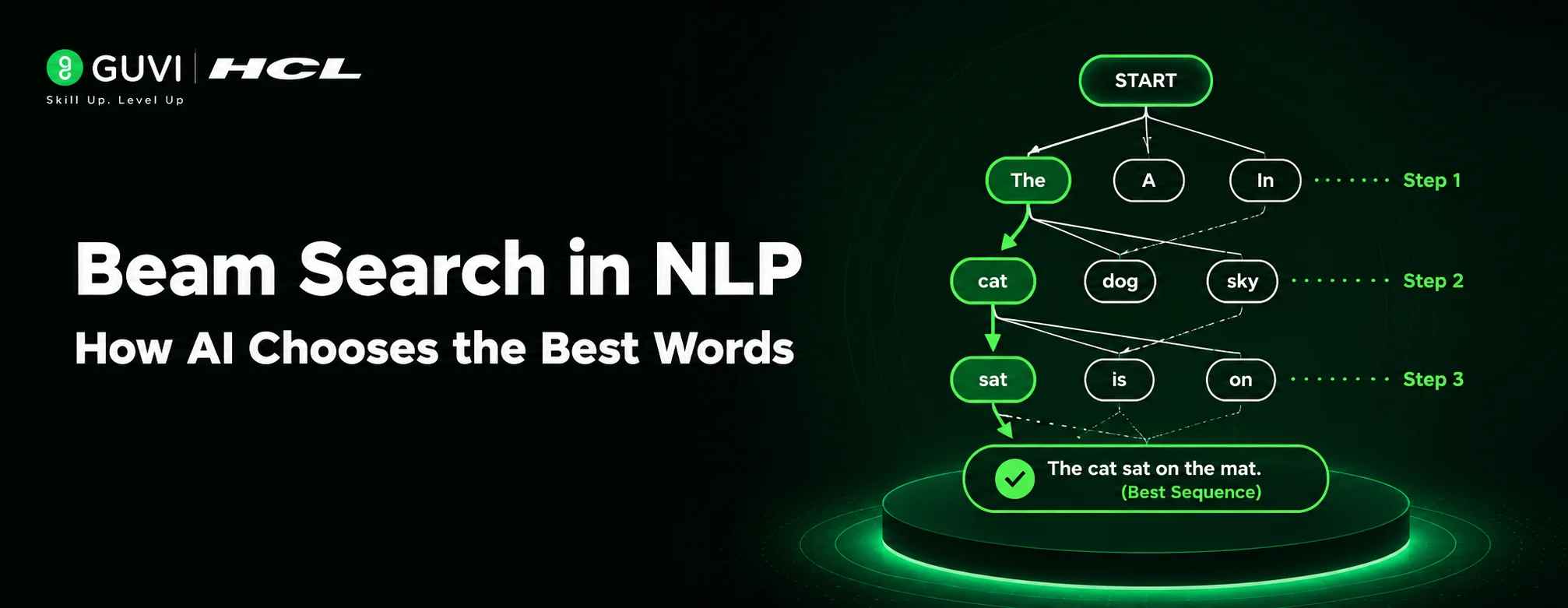
Step-by-Step Execution

1. Step 1: Initialise: Start with an empty sequence. Compute probabilities for all vocabulary tokens as the first word. Retain the top 2: e.g. [“The” (log-prob: −0.3), “A” (log-prob: −0.5)].
2. Step 2: Expand: Extend each surviving beam with every vocabulary token. “The” produces 8 candidates (“The cat”, “The dog”, “The sat”, …). “A” produces 8 more. Score all 16 by cumulative log-probability. Retain the top 2: e.g. [“The cat” (−0.7), “The dog” (−0.9)].
3. Step 3: Continue to expand each top-2 beam again. “The cat” → “The cat sat”, “The cat ran”, etc. “The dog” → “The dog sat”, “The dog ran”, etc. Score all candidates. Retain the top 2.
4. Termination: Continue until both beams produce an end-of-sequence token or the maximum length is reached. Return the beam with the highest cumulative log-probability as the final output.

Scoring: Cumulative Log-Probability

Beam Search scores sequences using cumulative log-probability, the sum of the log probabilities of each token in the sequence. Log-probabilities are used rather than raw probabilities to avoid numerical underflow (multiplying many small fractions quickly approaches zero). Higher cumulative log-probability means a more probable sequence overall.

Beam Width: The Central Trade-Off in Beam Search

Beam width, often denoted k or B, is the single most important hyperparameter in Beam Search. It determines how many candidate sequences are kept alive at each decoding step, and it controls the fundamental trade-off between output quality and computational cost.

• Beam width = 1: Identical to greedy search. Fastest, lowest quality. No exploration of alternatives.
• Beam width 3–5: The most common range in practical NLP systems. Provides meaningful quality improvement over greedy at modest computational overhead. Standard in neural machine translation.
• Beam width 10–20: Used when output quality is critical and compute is available. Produces noticeably better translations and summaries. Diminishing returns begin to appear beyond this range.
• Beam width = V (full beam): Equivalent to breadth-first exhaustive search at each step. Computationally infeasible for real vocabulary sizes.

The Diminishing Returns of Wider Beams

Research has shown that beam width improvements plateau relatively quickly. In most NLP tasks, moving from k=1 to k=5 produces substantial quality gains. Moving from k=5 to k=10 produces smaller but still meaningful gains. Beyond k=10–20, improvements become marginal for most tasks. This is why beam widths of 4–10 dominate practical deployments.

Length Normalisation

A known issue with standard Beam Search is a bias toward shorter sequences. Cumulative log-probabilities become more negative with every token added, making shorter sequences appear more probable simply because they have fewer terms. Length normalisation divides the cumulative log-probability by the sequence length (raised to a normalisation exponent α, typically 0.6–0.7), correcting this bias and producing longer, more complete outputs.

Real-World Applications of Beam Search in NLP and AI

Beam Search is not a research curiosity; it is the standard decoding algorithm in production NLP systems worldwide. Its combination of quality improvement over greedy search and computational feasibility makes it the default choice across a wide range of AI text generation tasks.

• Machine Translation:  Beam Search is the standard decoder in neural machine translation systems, including Google Translate, DeepL, and Microsoft Translator. Beam widths of 4–8 are typical. The algorithm ensures that translations are fluent and complete rather than cutting off or making locally greedy word choices.
• Text Summarisation:  Abstractive summarisation models use Beam Search to generate concise, coherent summaries from long documents. Length normalisation is particularly important here to prevent the decoder from producing excessively short summaries that maximise probability but miss key content.
• Speech Recognition: Automatic Speech Recognition (ASR) systems use Beam Search over acoustic model outputs, combined with language model scores, to produce accurate transcripts. The beam integrates acoustic probabilities and linguistic plausibility at each decoding step.
• Image Captioning:  Vision-language models that generate text descriptions of images use Beam Search to produce grammatically correct and semantically accurate captions. The beam ensures the caption describes the full image content rather than committing early to a partial description.
• Code Generation:  AI coding assistants like GitHub Copilot use variants of Beam Search and sampling to generate code completions. Beam Search ensures syntactically valid and logically coherent code sequences rather than random token-by-token greedy completions.

Limitations of Beam Search You Should Understand

• Output repetition:  Beam Search can produce repetitive text, especially in long-form generation, because high-probability token sequences tend to loop back to familiar patterns. Repetition penalties (applied to already-generated tokens) and diverse beam variants mitigate this.
• Low output diversity:  The top-k beams often converge on very similar sequences. This is acceptable for translation but problematic for creative generation, dialogue systems, and any task where diverse outputs are desired. Sampling-based methods produce more variety.
• Short sequence bias:  Without length normalisation, Beam Search favours shorter sequences. This must be explicitly corrected with length normalisation or a length penalty parameter.
• Computational cost grows with beam width:  Each doubling of beam width approximately doubles inference cost. For latency-sensitive applications, real-time translation, voice assistants, and wide beams may not be deployable without dedicated hardware optimisation.
• Not guaranteed optimal:  Despite being better than greedy search, Beam Search is still a heuristic; it does not guarantee finding the globally highest-probability sequence. It finds an approximation that is good enough for most practical purposes.

If you want to learn more about building skills for Claude Code and automating your procedural knowledge, do not miss the chance to enrol in HCL GUVI’s Intel & IITM Pravartak Certified Artificial Intelligence & Machine Learning courses. Endorsed with Intel certification, this course adds a globally recognised credential to your resume, a powerful edge that sets you apart in the competitive AI job market.

Conclusion

Beam Search occupies a uniquely important position in natural language processing and AI text generation: it is simple enough to implement efficiently, powerful enough to produce high-quality outputs, and flexible enough to adapt to a wide range of sequence generation tasks through variants like diverse beams, constrained decoding, and length normalisation.

The core insight that maintaining multiple hypotheses simultaneously and pruning aggressively at each step gives far better results than committing to a single path is elegant and practically impactful. From the Google Neural Machine Translation system to modern code generation assistants, Beam Search is the decoding workhorse of production NLP.

Understanding Beam Search deeply its mechanics, its beam width trade-offs, its failure modes, and its variants is essential for anyone building, evaluating, or deploying AI text generation systems. It is not the final word in sequence decoding, but it remains the standard against which all alternatives are measured.

FAQs

1. What is Beam Search in natural language processing?

Beam Search is a heuristic search algorithm used in sequence generation tasks in NLP. It maintains a fixed number of candidate sequences in the beam at each decoding step, expanding only the most promising ones rather than exploring every possible output or committing greedily to the single best token.

2. What is the difference between greedy search and Beam Search?

Greedy search selects the single highest-probability token at each step, fast but suboptimal, since locally best choices often lead to globally poor sequences. Beam Search keeps the top-k sequences at each step, exploring multiple paths simultaneously. 

3. What does beam width mean,n, and how do you choose it?

Beam width (k or B) is the number of candidate sequences kept alive at each decoding step. Larger beam widths produce better-quality outputs by exploring more of the sequence space, but increase computational cost proportionally. 

4. Why does Beam Search favour shorter sequences, and how is it fixed?

Beam Search scores sequences using cumulative log-probabilities, sums of negative numbers that become more negative as the sequence grows. This makes shorter sequences appear more probable simply because they accumulate fewer negative terms.

5. When should you use sampling instead of Beam Search?

Beam Search is optimal for tasks where there is a well-defined correct or near-correct output, such as machine translation, summarisation, speech recognition, and structured text generation. Sampling (top-k, nucleus/top-p) is preferable for open-ended creative tasks.