


Data Structure Articles
Sliding Window Technique: Explained with Examples
Two Pointer Technique: Problems and Applications


Get In Touch For Details! Request More Information

Adjacency matrix meaning and definition in DSA
Sep 15, 2026 11 Min Read 3693 Views
(Last Updated)
Ever tried to represent a social network, a road map, or a set of webpages linking to each other, and wondered how a computer actually stores all those connections? That’s exactly the problem graphs solve, and the adjacency matrix is one of the simplest, most direct ways to represent them.
An adjacency matrix is a two-dimensional array of size V×V that represents a graph, where each cell indicates whether an edge exists between the corresponding pair of vertices.
It’s one of the two standard ways to store a graph in memory, offering instant edge lookups in exchange for higher memory usage.
This guide covers what an adjacency matrix actually is, how to build and maintain one in Python, when to use it over an adjacency list, and the interview questions it shows up in most often.
Table of contents
- TL;DR Summary
- What Is an Adjacency Matrix?
- Why Use an Adjacency Matrix?
- Adjacency Matrix vs Adjacency List
- How to Create and Maintain an Adjacency Matrix
- Initialization
- Adding an Edge
- Removing an Edge
- Checking if an Edge Exists
- Iterating Through Neighbors
- Python Example
- Adjacency Matrix Implementation in Python With BFS and DFS
- Output
- How BFS Works With an Adjacency Matrix
- How DFS Works With an Adjacency Matrix
- Adjacency Matrix for Weighted vs Unweighted Graphs
- Unweighted Adjacency Matrix
- Weighted Adjacency Matrix
- Weighted Matrix Example in Python
- Matrix Exponentiation: Counting Paths of Length K
- Algorithms That Commonly Use Adjacency Matrix
- Time and Space Complexity
- Sparse vs Dense Graphs: Which Representation Should You Choose?
- Sparse Graph
- Dense Graph
- How to Choose
- Common Pitfalls and How to Avoid Them
- Advantages and Disadvantages
- Advantages
- Disadvantages
- Real-World Examples and Use Cases
- Where to Practice Adjacency Matrix Problems
- Adjacency Matrix Interview Questions With Solutions
- What Is the Space Complexity of an Adjacency Matrix?
- Why Is an Adjacency Matrix Symmetric for an Undirected Graph?
- How Do You Count Edges in an Undirected Adjacency Matrix?
- How Do You Count Edges in a Directed Adjacency Matrix?
- How Can You Detect a Self-Loop?
- What Is the Time Complexity of BFS Using an Adjacency Matrix?
- How Can You Convert an Adjacency Matrix Into an Adjacency List?
- Which Representation Is Better for Floyd–Warshall?
- Can an Adjacency Matrix Represent Parallel Edges?
- When Should You Avoid an Adjacency Matrix?
- Conclusion
- What exactly is the adjacency matrix in DSA used for?
- When should I prefer an adjacency list over an adjacency matrix?
- How do weighted edges appear in the adjacency matrix?
- Can adjacency matrices handle directed graphs?
- Are there memory-efficient variants of adjacency matrix for large graphs?
TL;DR Summary
- What it is: a V×V table where each cell records whether two vertices are connected
- Core trade-off: O(1) edge lookup, but O(V²) memory regardless of how many edges actually exist
- Best suited for: dense graphs, and algorithms like Floyd-Warshall that check every vertex pair repeatedly
- Its main rival: the adjacency list, which is more memory-efficient for sparse graphs
- Where it shows up: BFS, DFS, shortest-path algorithms, and a recurring topic in DSA interviews
| Factor | Adjacency Matrix | Adjacency List |
|---|---|---|
| Space | O(V²) | O(V + E) |
| Check an edge | O(1) | O(degree of vertex) |
| Find neighbours | O(V) | O(degree of vertex) |
| Best suited for | Dense graphs | Sparse graphs |
What Is an Adjacency Matrix?
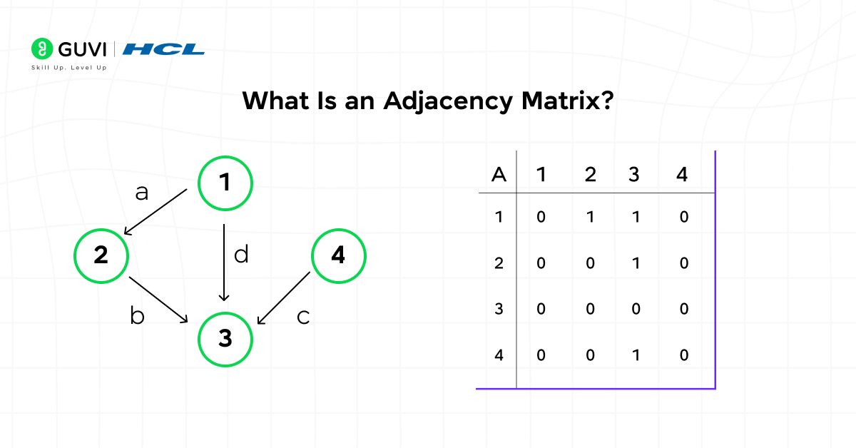
An adjacency matrix is a simple and structured way to represent a graph in programming. It is a two-dimensional array (N × N), where N is the total number of vertices (or nodes) in the graph. Each row and column of this matrix represents a vertex, and the value stored at any cell shows whether there is a connection (edge) between two vertices.
In simple words, an adjacency matrix tells us which nodes are connected to which, and how they are connected. This makes it one of the easiest ways to store and visualize relationships in a graph.
Here’s how it works:
- For unweighted graphs, the adjacency matrix contains 1 if there is an edge between two vertices and 0 if there is no edge.
- For weighted graphs, instead of using 1 and 0, we store the weight or cost of the edge. If no edge exists, we usually mark it as 0, -1, or INF (infinity).
- In directed graphs, the direction of the edge matters. So, if there is an edge from A to B, the value at matrix[A][B] will be 1, but matrix[B][A] might still be 0.
- In undirected graphs, the connections are two-way. That means the adjacency matrix is symmetric — if matrix[A][B] = 1, then matrix[B][A] = 1 too.
The main advantage of using an adjacency matrix is that it allows you to quickly check if an edge exists between two nodes in constant time O(1). This makes it highly efficient for operations where fast edge lookup is required, such as in graph traversal or shortest-path algorithms.
In short, an adjacency matrix in DSA is like a table that keeps track of all possible connections in a graph — making it easier to perform computations, analyze structures, and build algorithms efficiently.
Why Use an Adjacency Matrix?
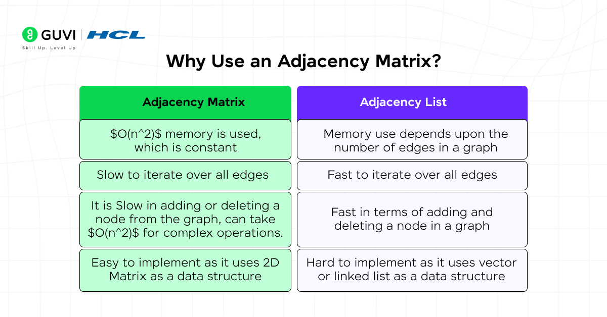
An adjacency matrix is one of the most efficient ways to represent a graph when you need quick access to connections between nodes. It provides a clear, table-like structure that allows fast and direct checking of whether an edge exists between any two vertices.
You should use an adjacency matrix in the following situations:
- When you need fast edge checks:
If you often need to verify whether two nodes are connected, an adjacency matrix is perfect. You can find this information instantly in O(1) time because each cell directly stores the connection status. - When the graph is dense:
A graph is called dense when it has many edges — close to the total possible number of edges (N²). In such cases, using an adjacency matrix makes sense because most cells in the matrix will contain valid connections, making the memory usage worthwhile. - When your algorithm relies on quick lookups:
Some algorithms, like the Floyd–Warshall algorithm (used to find shortest paths between all pairs of vertices), perform operations on every pair of nodes. The adjacency matrix works best here because it allows immediate access to every connection without searching through lists.
However, there’s one major drawback: an adjacency matrix always takes up O(N²) space. This means that even if your graph has very few connections (a sparse graph), the matrix still occupies memory for every possible pair of vertices. So while it’s excellent for dense graphs and quick lookups, it’s not memory-efficient for large or sparse graphs.
To truly understand why and when to use an adjacency matrix, learning the core data structures and algorithms behind it is essential. HCL GUVI’s DSA eBook helps you master these basics — from arrays and matrices to graphs and dynamic programming — with clear explanations, real examples, and practice questions. It’s an ideal companion for beginners and interview aspirants who want to build strong graph fundamentals.
Adjacency Matrix vs Adjacency List
An adjacency matrix stores every possible connection between vertices. An adjacency list stores only the connections that actually exist.
| Operation | Adjacency Matrix | Adjacency List |
| Space complexity | O(V²) | O(V + E) |
| Add an edge | O(1) | O(1) amortised |
| Remove an edge | O(1) | O(degree of vertex) |
| Check whether an edge exists | O(1) | O(degree of vertex) |
| Find all neighbours | O(V) | O(degree of vertex) |
| BFS or DFS traversal | O(V²) | O(V + E) |
| Best use case | Dense graphs with frequent edge checks | Sparse graphs with fewer connections |
The adjacency matrix is useful when the graph contains many edges or the algorithm repeatedly checks whether two vertices are connected.
The adjacency list is better when the graph contains fewer edges. It avoids allocating memory for connections that do not exist.
How to Create and Maintain an Adjacency Matrix
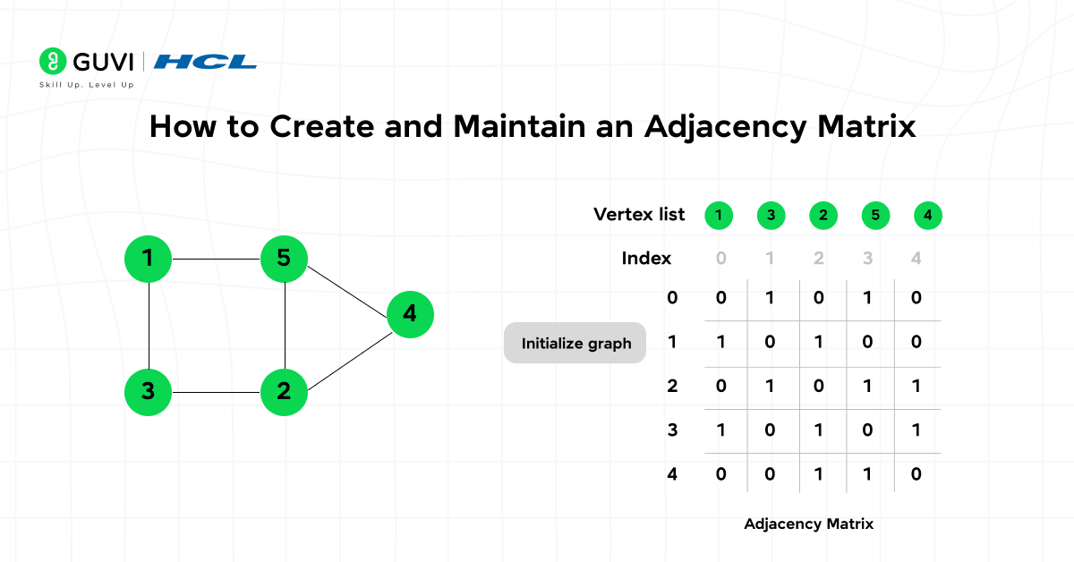
An adjacency matrix is one of the most popular and easy-to-understand ways to represent a graph in programming. Whether you are working with a simple unweighted graph or a complex weighted and directed one, understanding how to create, update, and maintain an adjacency matrix is an essential DSA skill.
Let’s break down the entire process step by step using simple terms, clear explanations, and practical code examples.
1. Initialization
The first step in creating an adjacency matrix is initializing the structure.
If a graph has N vertices, you’ll need an N × N matrix (a two-dimensional array) where each cell represents a possible connection between two nodes.
- For unweighted graphs:
You can initialize every cell with 0, meaning “no edge exists.”
When you add an edge between two nodes, you’ll change the corresponding entries to 1. - For weighted graphs:
You usually initialize every cell with a large number like INF (infinity) or sometimes -1 to indicate “no connection.”
If the graph allows self-loops, set the diagonal entries (where a node connects to itself) to 0 since the distance from a node to itself is zero.
This setup makes it easy to modify and check connections later.
2. Adding an Edge
Once your matrix is initialized, you can add an edge between two vertices.
- For an undirected graph:
Since the connection goes both ways, you must update both [u][v] and [v][u] entries to 1 (or to the edge weight in case of weighted graphs). - For a directed graph:
The edge goes in one direction, so you only update [u][v] and leave [v][u] unchanged.
Adding an edge takes O(1) time — meaning it’s instant, regardless of how large your graph is.
3. Removing an Edge
To remove an edge, simply reset the corresponding entries in the matrix:
- In an unweighted graph, set the value back to 0.
- In a weighted graph, set it to INF or -1 again to show that no edge exists.
This operation also takes O(1) time.
4. Checking if an Edge Exists
The biggest advantage of an adjacency matrix is how fast you can check whether an edge exists between two nodes.
You just look at the cell [u][v]:
- If it’s 1 (or any valid weight), an edge exists.
- If it’s 0 (or INF), no connection exists.
This check happens in constant time O(1) — one of the key reasons adjacency matrices are used in graph algorithms that require frequent lookups.
5. Iterating Through Neighbors
To find all the neighbors (connected vertices) of a particular node, you can scan its entire row in the matrix.
For example, to find all nodes connected to vertex u, check every column in row u and collect the indices where a connection exists (matrix[u][v] == 1).
This takes O(N) time per vertex because you have to check every possible node once.
6. Python Example
Before jumping into the code, let’s understand what unweighted and weighted graphs mean.
- Unweighted Graph: In an unweighted graph, every edge is treated equally. It only shows whether a connection exists or not — there’s no concept of distance or cost. For example, if cities are connected by roads but we don’t care about how long the roads are, it’s an unweighted graph.
- Weighted Graph: In a weighted graph, every edge has a specific value (weight) that represents cost, distance, or strength of connection. For example, if roads between cities have distances in kilometers, the distance becomes the weight of the edge.
1. Python code for unweighted graph
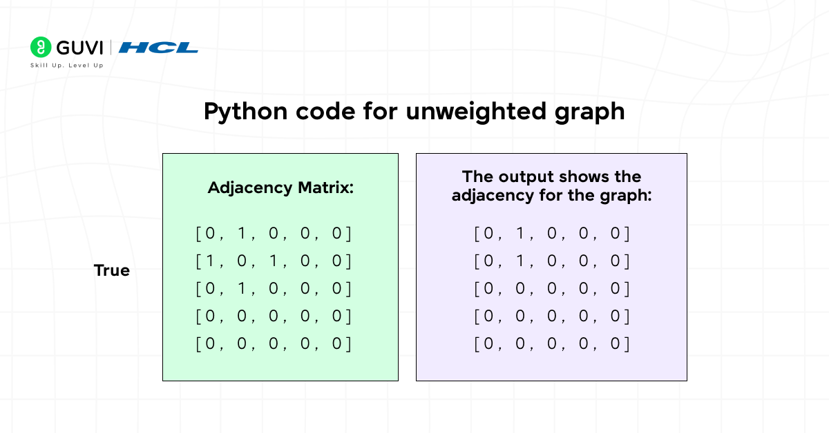
# Adjacency matrix for unweighted undirected graph
N = 5
adj = [[0] * N for _ in range(N)]

def add_edge(u, v):
    adj[u][v] = 1
    adj[v][u] = 1  # undirected graph

def remove_edge(u, v):
    adj[u][v] = 0
    adj[v][u] = 0

def has_edge(u, v):
    return adj[u][v] == 1

# Example usage
add_edge(0, 1)
add_edge(1, 2)
print(has_edge(0, 1))  # True
print(adj)
This code demonstrates how to add, remove, and check edges in a simple graph structure.
2. Python code for weighted graph
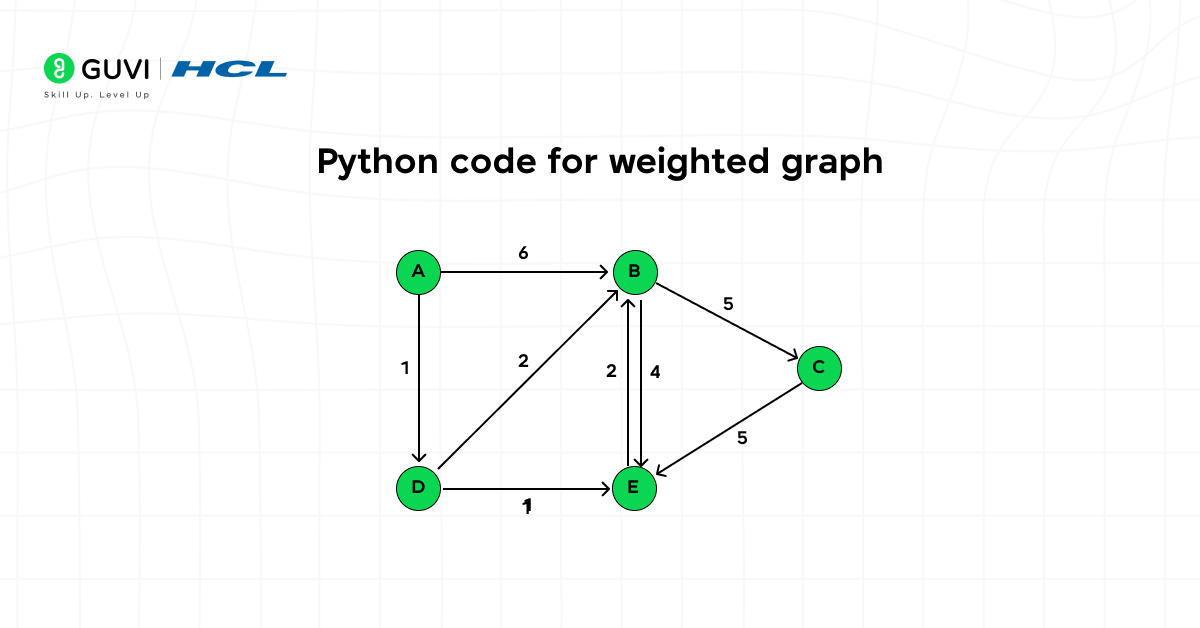
If your graph has weights and directions, you can use the following version:
INF = 10**9  # a large number representing 'no edge'
N = 4
adj = [[INF] * N for _ in range(N)]

for i in range(N):
    adj[i][i] = 0  # distance from a node to itself

def add_edge(u, v, w):
    adj[u][v] = w  # directed edge from u to v with weight w

# Example edges
add_edge(0, 1, 5)
add_edge(1, 2, 3)

# Example: adj[0][1] == 5, adj[1][0] == INF
This version is ideal for algorithms like Dijkstra or Floyd–Warshall that use edge weights.
Adjacency Matrix Implementation in Python With BFS and DFS
The following implementation creates an unweighted graph using an adjacency matrix. It supports directed and undirected graphs.
from collections import deque


class GraphMatrix:
    def __init__(self, vertices: int, directed: bool = False):
        if vertices <= 0:
            raise ValueError("The number of vertices must be greater than zero.")

        self.vertices = vertices
        self.directed = directed
        self.matrix = [
            [0] * vertices
            for _ in range(vertices)
        ]

    def _validate_vertex(self, vertex: int) -> None:
        if not 0 <= vertex < self.vertices:
            raise IndexError(
                f"Vertex must be between 0 and {self.vertices - 1}."
            )

    def add_edge(self, source: int, destination: int) -> None:
        self._validate_vertex(source)
        self._validate_vertex(destination)

        self.matrix[source][destination] = 1

        if not self.directed:
            self.matrix[destination][source] = 1

    def remove_edge(self, source: int, destination: int) -> None:
        self._validate_vertex(source)
        self._validate_vertex(destination)

        self.matrix[source][destination] = 0

        if not self.directed:
            self.matrix[destination][source] = 0

    def has_edge(self, source: int, destination: int) -> bool:
        self._validate_vertex(source)
        self._validate_vertex(destination)

        return self.matrix[source][destination] == 1

    def bfs(self, start: int) -> list[int]:
        self._validate_vertex(start)

        visited = [False] * self.vertices
        traversal_order = []
        queue = deque([start])

        visited[start] = True

        while queue:
            current_vertex = queue.popleft()
            traversal_order.append(current_vertex)

            for neighbour, connected in enumerate(
                self.matrix[current_vertex]
            ):
                if connected and not visited[neighbour]:
                    visited[neighbour] = True
                    queue.append(neighbour)

        return traversal_order

    def dfs(self, start: int) -> list[int]:
        self._validate_vertex(start)

        visited = [False] * self.vertices
        traversal_order = []

        def visit(vertex: int) -> None:
            visited[vertex] = True
            traversal_order.append(vertex)

            for neighbour, connected in enumerate(
                self.matrix[vertex]
            ):
                if connected and not visited[neighbour]:
                    visit(neighbour)

        visit(start)
        return traversal_order

    def display(self) -> None:
        for row in self.matrix:
            print(row)


graph = GraphMatrix(vertices=5)

graph.add_edge(0, 1)
graph.add_edge(0, 2)
graph.add_edge(1, 3)
graph.add_edge(2, 4)

print("Adjacency matrix:")
graph.display()

print("BFS traversal:", graph.bfs(0))
print("DFS traversal:", graph.dfs(0))
Output
Adjacency matrix:
[0, 1, 1, 0, 0]
[1, 0, 0, 1, 0]
[1, 0, 0, 0, 1]
[0, 1, 0, 0, 0]
[0, 0, 1, 0, 0]

BFS traversal: [0, 1, 2, 3, 4]
DFS traversal: [0, 1, 3, 2, 4]
How BFS Works With an Adjacency Matrix
BFS uses a queue to visit vertices level by level. The algorithm scans the complete matrix row of every visited vertex to find its neighbours.
Its time complexity is O(V²), even when the graph contains only a few edges.
How DFS Works With an Adjacency Matrix
DFS follows one connection as deeply as possible before backtracking. The recursive implementation scans each vertex row to find unvisited neighbours.
Its time complexity is also O(V²) with an adjacency matrix.
Adjacency Matrix for Weighted vs Unweighted Graphs
The values stored inside the matrix depend on whether the graph is weighted or unweighted.
Unweighted Adjacency Matrix
An unweighted graph records only whether an edge exists.
- Store
1when two vertices are connected. - Store
0when no edge exists.
Consider the following matrix:
0 1 1
1 0 0
1 0 0
Vertex 0 connects to vertices 1 and 2. The matrix does not provide any information about distance or cost.
Weighted Adjacency Matrix
A weighted graph stores the cost, distance, or value associated with each edge.
0   5   8
5   0  INF
8  INF  0
This matrix shows:
- The edge between vertices 0 and 1 has a weight of 5.
- The edge between vertices 0 and 2 has a weight of 8.
- No direct edge exists between vertices 1 and 2.
Use INF, None, or another clear marker for a missing edge. Using 0 can create confusion when the graph permits valid zero-weight edges.
Weighted Matrix Example in Python
INF = float("inf")
vertices = 4

matrix = [
    [INF] * vertices
    for _ in range(vertices)
]

for vertex in range(vertices):
    matrix[vertex][vertex] = 0


def add_weighted_edge(
    source: int,
    destination: int,
    weight: int,
    directed: bool = False
) -> None:
    matrix[source][destination] = weight

    if not directed:
        matrix[destination][source] = weight


add_weighted_edge(0, 1, 5)
add_weighted_edge(0, 2, 8)
add_weighted_edge(1, 3, 4)

for row in matrix:
    print(row)
Weighted adjacency matrices work naturally with algorithms such as Floyd–Warshall. They can also support dense-graph versions of Prim’s and Dijkstra’s algorithms.
BFS and DFS can still traverse a weighted graph, but they do not use the edge weights while deciding the traversal order.
Matrix Exponentiation: Counting Paths of Length K
One genuinely underused application of the adjacency matrix: raising it to a power lets you count paths of an exact length between any two vertices, a trick that comes up in competitive programming and certain interview questions.
If A is your adjacency matrix, then A² gives the number of paths of length 2 between every pair of vertices, A³ gives paths of length 3, and so on.
def matrix_multiply(A, B):
    n = len(A)
    result = [[0] * n for _ in range(n)]
    for i in range(n):
        for j in range(n):
            for k in range(n):
                result[i][j] += A[i][k] * B[k][j]
    return result

def count_paths_of_length_k(adj_matrix, k):
    n = len(adj_matrix)
    result = [[1 if i == j else 0 for j in range(n)] for i in range(n)]
    base = adj_matrix
    while k > 0:
        if k % 2 == 1:
            result = matrix_multiply(result, base)
        base = matrix_multiply(base, base)
        k //= 2
    return result

# Triangle graph: 0-1, 1-2, 2-0
adj = [
    [0, 1, 1],
    [1, 0, 1],
    [1, 1, 0]
]

print(count_paths_of_length_k(adj, 2))
# [[2, 1, 1], [1, 2, 1], [1, 1, 2]]
Explanation: this uses fast exponentiation by squaring, computing A^k in O(log k) matrix multiplications instead of k of them.

For the triangle graph above, there are 2 paths of length 2 from any vertex back to itself (go to either neighbor and return), and 1 path of length 2 between any two distinct vertices (via the third vertex).
Algorithms That Commonly Use Adjacency Matrix
- Floyd-Warshall (All Pairs Shortest Path) — natural with matrix inputs.
- Some implementations of Prim’s algorithm for dense graphs use an adjacency matrix.
- Graph algorithms that rely on repeated constant time edge checks.
- Matrix power methods for counting paths of length k (using repeated matrix multiplication).
Time and Space Complexity
Let’s understand how efficient an adjacency matrix really is:
- Space Complexity: O(N²)
Each vertex pair requires a cell, so memory usage grows with the square of the number of vertices. - Check if edge exists: O(1)
You can check for a connection instantly. - Add or remove an edge: O(1)
Just update one or two entries. - Iterate through all neighbors of a node: O(N)
You must scan the entire row. - Iterate through all edges: O(N²)
You’ll need to check every cell of the matrix.
This means adjacency matrices are best suited for dense graphs, where the number of edges (E) is close to N². For sparse graphs (where there are far fewer edges), adjacency lists are usually more memory-efficient.
Sparse vs Dense Graphs: Which Representation Should You Choose?
A sparse graph has significantly fewer edges than the maximum possible number. A dense graph contains a large proportion of all possible edges.
Sparse Graph
A sparse graph follows this general relationship:
E is much smaller than V²Examples include:
- Road networks
- Website links
- Social networks with millions of users
- Dependency graphs
An adjacency list is usually better because it stores only existing edges.
Dense Graph
A dense graph contains edges close to the maximum possible number.
For a simple undirected graph, the maximum number of edges is:
V × (V - 1) / 2For a simple directed graph, the maximum is:
V × (V - 1)Examples may include:
- Small fully connected networks
- Complete communication systems
- Graphs used in all-pairs shortest-path problems
An adjacency matrix becomes more practical because most matrix cells contain useful information.
How to Choose
Use an adjacency matrix when:
- The graph is dense.
- The number of vertices is manageable.
- Constant-time edge checks are important.
- The algorithm processes most vertex pairs.
- Matrix-based operations are required.
Use an adjacency list when:
- The graph is sparse.
- The graph contains many vertices.
- Memory efficiency is important.
- The algorithm frequently visits neighbours.
- BFS or DFS performance is a priority.
There is no universal density point at which one representation becomes better. The choice also depends on the programming language, memory limits, and operations performed most frequently.
Common Pitfalls and How to Avoid Them
- Using a matrix for very large graphs. Avoid an adjacency matrix when the vertex count is large (for example, past 10,000 vertices) unless the graph is genuinely dense, memory usage will explode.
- Assuming symmetry without checking. For directed graphs, don’t assume matrix[u][v] equals matrix[v][u].
- Memory allocation overhead. In languages like Python, a list of lists carries overhead per list, consider NumPy arrays or bitsets for more compact storage when performance matters.
Advantages and Disadvantages
Advantages
- Constant-time edge lookup, O(1).
- Simple to implement.
- Easy to convert to matrices used in algorithms (for example, matrix multiplication interpretations of graph problems).
- Works naturally with linear algebra and matrix-based graph algorithms.
Disadvantages
- Space-inefficient for large vertex counts and sparse graphs.
- Scanning neighbors requires O(N) time even if a node has very few neighbors.
- Not suitable for very large graphs (millions of nodes).
Real-World Examples and Use Cases
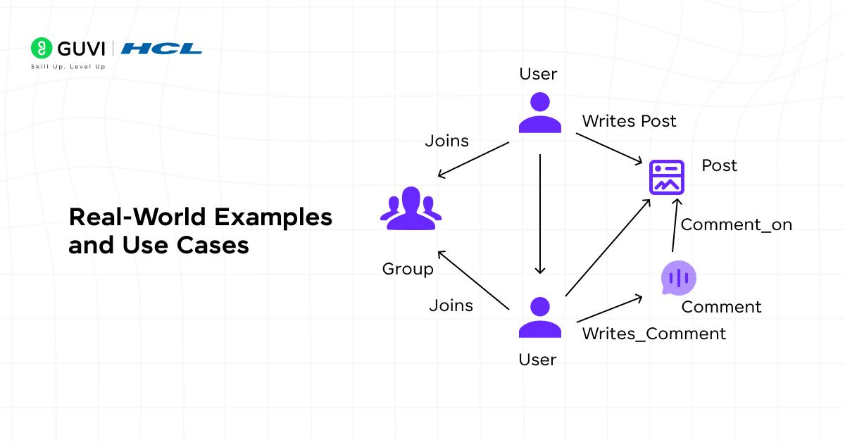
The adjacency matrix is not just an abstract DSA topic — it’s something that appears in many real-life systems we use every day. Here are some simple, relatable examples that show where and how adjacency matrices can be applied:
1. Social Media Friendships
Imagine you have a small group of friends on a social media app. Each person can follow or be friends with others.
If you make a table where both rows and columns represent people, and you mark a 1 wherever two people are connected, that table is an adjacency matrix.
For example:
- If Alice and Bob are friends, you’ll have a 1 at Alice → Bob and Bob → Alice.
- If Alice is not connected to John, that cell stays 0.
This makes it easy for the app to instantly check who is connected to whom.
2. City Map or Road Network
Think about a few cities connected by roads — for instance, Chennai, Bengaluru, and Hyderabad.
Each city can be a vertex, and each road can be an edge.
- If a direct road connects Chennai to Bengaluru, mark it as 1.
- If there’s no direct road between Chennai and Hyderabad, mark it as 0.
If you include distances (like 350 km between two cities), you can use weights in the matrix instead of just 1 and 0. This helps navigation apps quickly find the shortest routes between places.
3. Airline Flight Routes
Airlines use adjacency matrices to manage direct flight routes between airports.
- If there’s a direct flight from Delhi to Mumbai, mark that as 1.
- If there’s no direct flight between two cities, it stays 0.
When you add flight durations or costs as weights, it becomes easy to calculate the shortest or cheapest route.
4. Classroom Connections or Team Projects
Imagine you have five students working together on different projects. Some students collaborate often, while others don’t.
You can make an adjacency matrix where:
- Each student is a row and column.
- A 1 means they’ve worked together.
- A 0 means they haven’t.
This helps visualize group dynamics or teamwork patterns — similar to how project managers track collaborations.
5. Internet or Computer Networks
When multiple computers are connected in a small office network, each device is a node, and each cable or Wi-Fi link is an edge.
The adjacency matrix can show which computers can directly communicate. This is useful for network troubleshooting or data transfer optimization.
In short, the adjacency matrix helps us model and manage relationships — whether between people, cities, airports, students, or computers. It’s a simple yet powerful way to represent real-world connections clearly and efficiently.
Where to Practice Adjacency Matrix Problems
Reading through the theory only gets you so far, these platforms let you actually build and test graph problems using an adjacency matrix.
- LeetCode: a large collection of graph problems tagged specifically by difficulty, many of which are naturally solved with an adjacency matrix, including several of the shortest-path and dense-graph problems covered in this guide.
- HackerRank: structured graph theory practice with a difficulty progression, useful for building confidence with BFS and DFS implementations before moving to timed contests.
- Codeforces: genuinely challenging, competitive-programming-level graph problems once you’re comfortable with the fundamentals, useful for practicing matrix exponentiation and dense-graph algorithms specifically.
Adjacency Matrix Interview Questions With Solutions
1. What Is the Space Complexity of an Adjacency Matrix?
Answer:
An adjacency matrix requires O(V²) space because it stores one cell for every possible pair of vertices.
A graph containing 1,000 vertices requires a matrix with 1,000,000 cells, even when only a few edges exist.
2. Why Is an Adjacency Matrix Symmetric for an Undirected Graph?
Answer:
Every undirected edge connects both vertices in both directions.
An edge between vertices u and v causes:
matrix[u][v] = 1
matrix[v][u] = 1
The values above and below the main diagonal therefore match.
A directed graph does not require this symmetry.
3. How Do You Count Edges in an Undirected Adjacency Matrix?
Answer:
Add all values in the matrix and divide the result by two. Every edge appears twice in an undirected graph.
def count_undirected_edges(matrix: list[list[int]]) -> int:
    total = sum(sum(row) for row in matrix)
    return total // 2
This solution assumes that the graph does not contain self-loops.
A self-loop appears on the main diagonal and should be counted only once.
4. How Do You Count Edges in a Directed Adjacency Matrix?
Answer:
Add all values in the matrix. A directed edge appears only once.
def count_directed_edges(matrix: list[list[int]]) -> int:
    return sum(sum(row) for row in matrix)
This approach works for an unweighted matrix containing 0 and 1.
5. How Can You Detect a Self-Loop?
Answer:
A self-loop exists when a vertex connects to itself. Check the main diagonal of the matrix.
def has_self_loop(matrix: list[list[int]]) -> bool:
    return any(
        matrix[vertex][vertex] != 0
        for vertex in range(len(matrix))
    )
For weighted graphs, make sure the diagonal convention does not use 0 merely to represent the distance from a vertex to itself.
6. What Is the Time Complexity of BFS Using an Adjacency Matrix?
Answer:
The time complexity is O(V²).
BFS visits each vertex and scans a row containing V cells. It performs this row scan for up to V vertices.
With an adjacency list, BFS takes O(V + E).
7. How Can You Convert an Adjacency Matrix Into an Adjacency List?
Answer:
Scan every matrix cell and add the destination vertex whenever an edge exists.
def matrix_to_list(
    matrix: list[list[int]]
) -> list[list[int]]:
    adjacency_list = [
        [] for _ in range(len(matrix))
    ]

    for source, row in enumerate(matrix):
        for destination, connected in enumerate(row):
            if connected:
                adjacency_list[source].append(destination)

    return adjacency_list
The conversion requires O(V²) time because every cell must be checked.
8. Which Representation Is Better for Floyd–Warshall?
Answer:
An adjacency matrix is the natural choice for Floyd–Warshall.
The algorithm calculates shortest paths between every pair of vertices. It repeatedly reads and updates distances using matrix indices.
Its overall time complexity is O(V³), while its space complexity is O(V²).
9. Can an Adjacency Matrix Represent Parallel Edges?
Answer:
A standard binary adjacency matrix cannot distinguish multiple edges connecting the same pair of vertices.
A modified matrix can store the number of parallel edges:
matrix[u][v] = number of edgesA weighted graph with parallel edges may instead store the minimum edge weight or use a list of weights in each cell.
10. When Should You Avoid an Adjacency Matrix?
Answer:
Avoid it when the graph has many vertices but very few edges.
The matrix still allocates O(V²) memory. An adjacency list is usually more efficient for large road networks, dependency graphs, and social networks.
Conclusion
The adjacency matrix is one of the simplest and most powerful ways to represent graphs in DSA. It provides instant edge lookups and a clear structure that’s easy to understand and implement. Because of its O(N²) memory requirement, it works best for dense graphs, where most nodes are connected to each other. However, for very large or sparse graphs, it’s often better to use an adjacency list to save space.
Understanding how an adjacency matrix works — along with its strengths and limitations — helps you choose the right graph representation for your algorithm. Whether you’re working on pathfinding, network design, or graph traversal, mastering this concept lays a strong foundation for advanced topics like BFS, DFS, Dijkstra’s, and Floyd–Warshall algorithms.
If you want to gain practical experience in building and optimizing graph algorithms, consider joining the HCL GUVI’s DSA using python course as it offers mentor-led sessions, hands-on coding practice, and real-world projects that help you strengthen your DSA skills and become job-ready.
FAQs
1. What exactly is the adjacency matrix in DSA used for?
It stores connections between every pair of vertices in an N×NN \times NN×N grid. It is used to quickly test the presence of an edge between two nodes and to run matrix-friendly graph algorithms.
2. When should I prefer an adjacency list over an adjacency matrix?
Prefer adjacency lists when the graph is sparse (E≪N2E \ll N^2E≪N2), because lists use O(N+E)O(N + E)O(N+E) space, are more memory efficient, and neighbor iteration is proportional to degree.
3. How do weighted edges appear in the adjacency matrix?
Instead of 1 and 0, a weighted adjacency matrix stores the weight value in matrix[u][v], and a sentinel (like INF) when no edge exists.
4. Can adjacency matrices handle directed graphs?
Yes. For directed graphs the matrix is not necessarily symmetric; matrix[u][v] may differ from matrix[v][u].
5. Are there memory-efficient variants of adjacency matrix for large graphs?
Yes — bitsets, compressed sparse row (CSR), coordinate (COO) formats, and storing only upper/lower triangles for undirected graphs are common optimizations.
Success Stories

About the Author
Jebasta
I translate the language of data into stories that anyone can understand. As a writer with a data science background, I simplify analytics, AI, and decision-making so beginners and enthusiasts can confidently explore the world of data.
View all posts by Jebasta
Connect with me @














Did you enjoy this article?