

Artificial Intelligence and Machine Learning Articles
Role Prompting: How to Give Claude a Persona
Using Claude to Automate Customer FAQs


Get In Touch For Details! Request More Information
What is Gradient Descent in Machine Learning? A Beginner’s Guide 2025
Sep 24, 2025 6 Min Read 2832 Views
(Last Updated)
Gradient descent in machine learning is the backbone that powers the learning process for various algorithms, from simple linear regression to complex neural networks. When you’re first diving into ML concepts, understanding what gradient descent is and how it works becomes essential for your learning journey.
Simply put, gradient descent is an iterative optimization algorithm designed to find the local minimum of a function. This powerful technique helps minimize the cost function of machine learning models, therefore improving their accuracy and performance.
In this beginner-friendly guide, you’ll learn how gradient descent works, why it’s important, and how different variations of this algorithm can be applied to solve real-world problems. Let’s begin!
Table of contents
- What is Gradient Descent in Machine Learning?
- Why optimization is needed
- How Gradient Descent Works Step-by-Step
- Initialize parameters
- Compute predictions
- Calculate loss
- Compute gradients
- Update parameters
- Repeat until convergence
- Key Components of Gradient Descent
- 1) Cost function explained
- 2) Understanding gradients
- 3) Role of learning rate
- 4) Choosing the right learning rate
- Types of Gradient Descent Algorithms
- 1) Batch Gradient Descent
- 2) Stochastic Gradient Descent (SGD)
- 3) Mini-Batch Gradient Descent
- 4) Momentum and Nesterov
- 5) RMSprop and Adam
- Concluding Thoughts…
- FAQs
- Q1. What is gradient descent in machine learning?
- Q2. How does gradient descent work step-by-step?
- Q3. What are the different types of gradient descent algorithms?
- Q4. How do you choose the right learning rate for gradient descent?
- Q5. What are common challenges in gradient descent and how can they be addressed?
What is Gradient Descent in Machine Learning?
At its core, gradient descent stands as a powerful optimization algorithm that machine learning models rely on to find the best possible parameters. Unlike conventional approaches, this technique works by systematically minimizing a cost function through iterative adjustments.
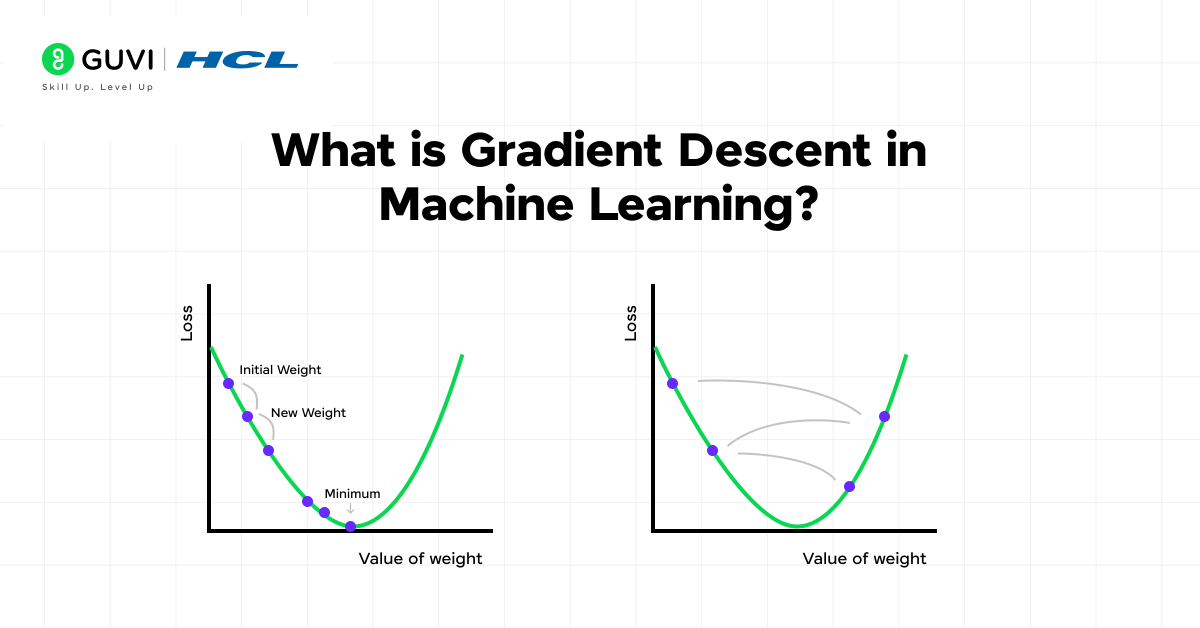
The process follows a simple yet effective approach:
- Start with initial parameter values
- Calculate the current prediction error (loss)
- Determine the direction to adjust parameters to reduce that loss
- Update the parameters accordingly
- Repeat until convergence
Essentially, a model has “converged” when additional iterations no longer significantly reduce the loss function value. At this point, the algorithm has discovered the optimal parameter values for the given data.
Why optimization is needed
Optimization sits at the very heart of machine learning. Without it, there would be no “learning” happening at all.
Machine learning models require optimization for several critical reasons:
- Parameter Refinement: Finding the ideal values for weights and biases that minimize prediction errors
- Accuracy Improvement: Lowering the gap between predicted and actual outputs
- Effective Performance: Ensuring models solve problems efficiently
The cost (or loss) function acts as a barometer that measures the difference between what your model predicts and the actual truth. As this function approaches zero, your model’s accuracy increases dramatically. Additionally, proper optimization helps prevent both underfitting (where models perform poorly on training data) and overfitting (where models perform well on training data but fail with new data).
How Gradient Descent Works Step-by-Step
The step-by-step process of gradient descent reveals the elegant simplicity behind this powerful optimization technique. While the mathematical concepts might initially seem complex, breaking down the algorithm into its fundamental steps makes it much easier to understand.
1. Initialize parameters
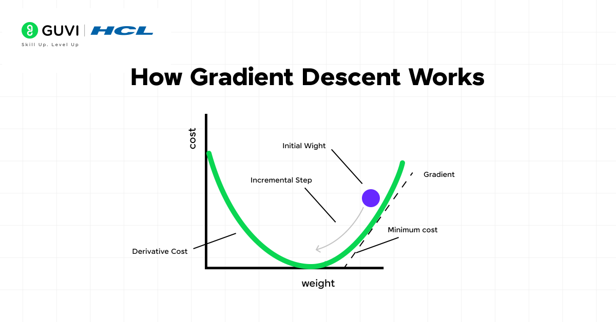
The gradient descent journey begins with parameter initialization. Generally, you start by assigning random small values to your model’s parameters (weights and biases). For simpler models like linear regression, this might involve setting initial values close to zero.
This initialization serves as your starting point on the “mountain” from which you’ll begin your descent. The quality of initialization matters, though it doesn’t need to be perfect – the algorithm will refine these values through iteration.
Key points to remember:
- Random initialization helps avoid getting stuck in suboptimal solutions
- In neural networks, specialized methods like Xavier initialization are often used
- The initial values provide a baseline for measuring improvement

2. Compute predictions
Once parameters are initialized, the next step involves using these parameters to make predictions. In this phase, your model generates outputs based on input features and current parameter values.
For instance, in linear regression, you’d compute: y_predicted = weight * x + bias, where x represents your input features, and the weight and bias are your initialized parameters.
3. Calculate loss
After generating predictions, you need to measure how far these predictions are from actual values. This measurement occurs through a loss function (also called a cost function).
The loss function quantifies the error between predicted and actual values. Common examples include:
- Mean Squared Error (MSE) for regression problems
- Cross-entropy loss for classification tasks
A higher loss value indicates poorer model performance. For example, calculating MSE might look like: (1/n) * Σ(y_true – y_predicted)².
4. Compute gradients
This step forms the heart of gradient descent. Here, you calculate the gradient of the loss function with respect to each parameter.
The gradient is essentially a vector that points in the direction of steepest ascent of the function. Furthermore, to minimize the loss, you need to move in the opposite direction of this gradient.
In simple terms, the gradient tells you:
- Which direction to adjust each parameter
- How much adjustment each parameter needs (magnitude)
For complex models, this calculation uses techniques like backpropagation.
5. Update parameters
With gradients calculated, it’s time to update your parameters. The update follows a simple yet powerful formula:
Parameter_new = Parameter_old – (Learning_rate * Gradient)
The learning rate controls how big each step should be. As illustrated in practical implementations:
- Too large a learning rate might cause overshooting and prevent convergence
- Too small a learning rate might result in unnecessarily slow progress
Common learning rates range between 0.001 and 0.3, though this depends on your specific problem.
6. Repeat until convergence
The final step involves repeating steps 2-5 until your model converges to an optimal solution. Convergence typically means either:
- The loss function has reached a minimum (or is close enough to it)
- Changes in parameters have become negligibly small
- A predetermined number of iterations has been completed
A model has successfully converged when additional iterations no longer significantly reduce the loss. This indicates you’ve found the (local) minimum of your cost function.
In practice, you might monitor the loss during training to determine when to stop. Meanwhile, various techniques like learning rate scheduling can help speed up convergence.
Key Components of Gradient Descent
Understanding the key components of gradient descent helps demystify how this optimization algorithm works in machine learning. By breaking it down into its core elements, you can grasp how models learn from data and improve over time.
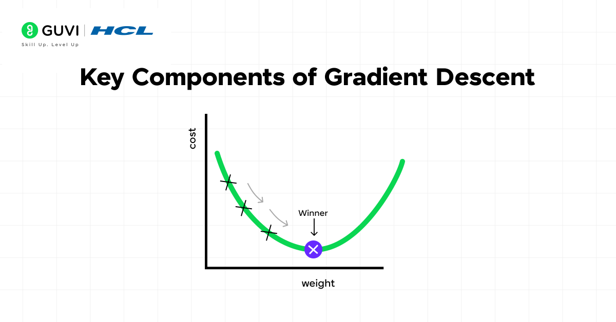
1) Cost function explained
The cost function (sometimes called the loss function) serves as the compass for gradient descent, guiding the algorithm toward optimal performance. It measures the difference between what your model predicts and the actual values in your training data. In essence, the cost function quantifies the error as a single real number that the algorithm works to minimize.
Common cost functions include:
- Mean Squared Error (MSE): Used primarily in regression problems, measuring the average squared difference between predictions and actual values
- Cross-Entropy Loss: Typically used in classification tasks, calculating the difference between actual and predicted probability distributions
When plotted, the cost function creates a surface with hills and valleys, where the algorithm’s goal is to find the lowest valley (minimum point).
2) Understanding gradients
A gradient is fundamentally the derivative of a function that has more than one input variable. In simpler terms, it represents the slope or steepness at a particular point on the cost function’s surface.
The gradient points in the direction of steepest ascent, so to minimize the cost function, the algorithm moves in the opposite direction. This mathematical insight forms the foundation of how gradient descent navigates toward optimal parameters.
Each component in the gradient vector is called a partial derivative, which assumes all other variables remain constant. These partial derivatives indicate how much each parameter contributes to the model’s error.
3) Role of learning rate
The learning rate controls how big a step the model takes in the direction of the negative gradient. It acts as a hyperparameter that determines the pace at which your model adjusts its parameters with each iteration.
This crucial component directly affects:
- Convergence speed: How quickly your model reaches its optimal state
- Stability: Whether your model can settle on the minimum or will overshoot it
The learning rate represents how much newly acquired information overrides old information, metaphorically showing the speed at which a machine learning model “learns”.
4) Choosing the right learning rate
Selecting an appropriate learning rate involves finding a delicate balance. A rate that’s too high might cause the model to overshoot the minimum point, leading to divergence or oscillations. Conversely, a rate that’s too low results in unnecessarily slow training that might get stuck in undesirable local minima.
Most common learning rates fall between 0.001 and 0.3, yet the ideal value depends on your specific problem. Several strategies exist for learning rate selection:
- Constant learning rate: Maintains the same rate throughout training
- Decay strategies: Begin with higher rates that gradually decrease
- Adaptive methods: Adjust rates automatically based on training progress
By understanding these key components, you gain deeper insight into how gradient descent finds optimal solutions for machine learning problems.
Here are a couple of surprising tidbits about gradient descent that you might not know:
Inspired by Nature: The concept of gradient descent is closely related to how water flows downhill. Just like water naturally moves toward the lowest point in a valley, gradient descent iteratively adjusts parameters to “flow” toward the minimum of a cost function.
Used Beyond Machine Learning: While famous in ML, gradient descent is also widely applied in economics, physics, and even biology for solving optimization problems. Its versatility makes it one of the most powerful mathematical tools of the modern era.
These facts highlight how a simple mathematical idea has shaped not just machine learning, but countless scientific and engineering disciplines.
Types of Gradient Descent Algorithms
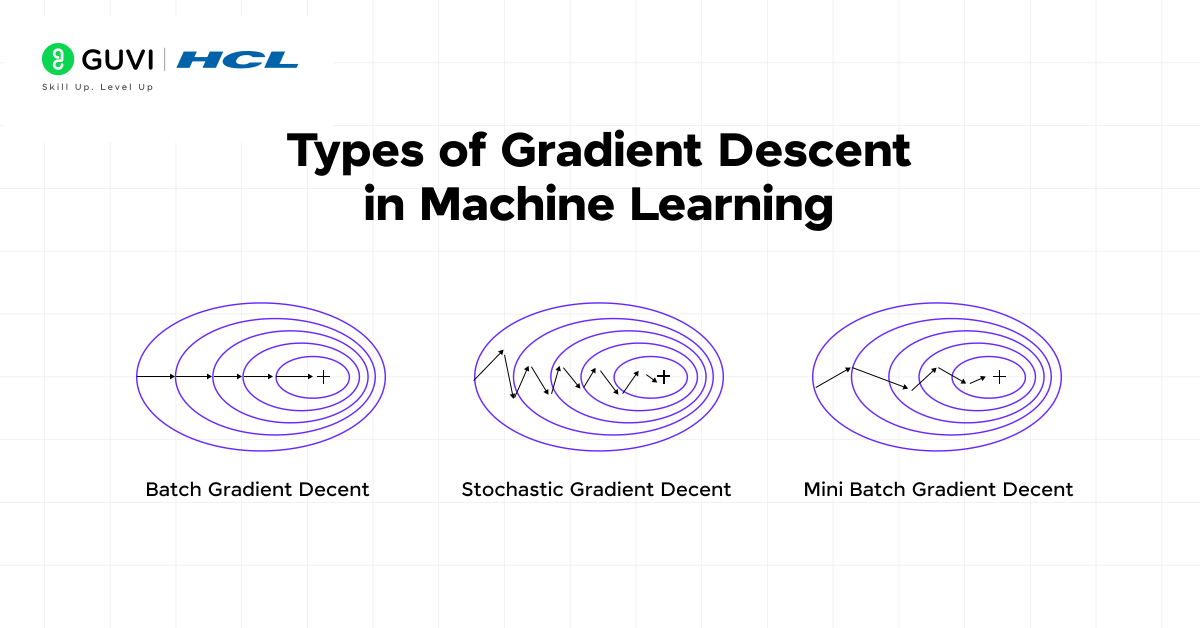
Gradient descent algorithms come in several variations, each with unique characteristics that make them suitable for different scenarios. These variants primarily differ in how much data they use for each parameter update cycle.
1) Batch Gradient Descent
Batch Gradient Descent processes the entire dataset before updating model parameters. This approach computes the gradient using all training examples at once, producing stable error gradients and consistent convergence. The algorithm makes just one update per epoch, resulting in predictable optimization paths.
Advantages:
- Provides precise gradient estimates for smooth error manifolds
- Offers stable and consistent convergence
However, batch gradient descent becomes impractical with large datasets due to high memory requirements and computational costs.
2) Stochastic Gradient Descent (SGD)
SGD updates model parameters after processing just one randomly selected training example at a time. Unlike batch methods, SGD makes frequent updates—once per training example.
Advantages:
- Significantly faster for large datasets
- Can escape local minima more effectively
- Supports online learning with continuous data streams
Despite its speed, SGD produces noisier gradients that can cause fluctuations during training.
3) Mini-Batch Gradient Descent
Mini-batch gradient descent strikes a balance between the previous approaches by using small subsets of data (typically 32-256 examples) for each update. This method has become the most common implementation in deep learning.
Advantages:
- Combines computational efficiency with stable convergence
- Enables effective use of hardware acceleration like GPUs
- Requires less memory than batch methods
4) Momentum and Nesterov
Momentum enhances gradient descent by accumulating past gradients, helping models overcome oscillations and navigate challenging loss landscapes. It acts like a ball rolling downhill, building velocity in consistent directions.
Nesterov momentum (NAG) improves this further by calculating gradients at projected positions rather than current ones. This creates a corrective effect that helps prevent overshooting minima.
5) RMSprop and Adam
RMSprop adapts learning rates for each parameter separately using an exponential moving average of squared gradients. This helps address the diminishing learning rate problem found in earlier methods.
Adam (Adaptive Moment Estimation) combines momentum’s velocity with RMSprop’s adaptive learning rates. It maintains both first and second moments of gradients, making it particularly effective for complex models with large datasets. Adam typically achieves superior results with minimal tuning.
Master AI & ML fundamentals like Gradient Descent with HCL GUVI’s IIT-M & Intel-powered AI/ML Course. Learn through real-world projects, live classes, and expert mentorship—designed to fast-track your career in AI.
Concluding Thoughts…
Gradient descent undoubtedly serves as the foundation for how machine learning algorithms learn from data. Throughout this guide, you’ve seen how this powerful optimization technique helps models find their best possible parameters through iterative improvement.
As you continue your machine learning journey, you’ll find gradient descent appearing across various algorithms—from simple linear regression to complex neural networks with millions of parameters. The concepts you’ve learned here will help you understand why models behave the way they do and how to improve their performance.
I hope this article has aided your learning journey, and if you have any doubts, do reach out to me through the comments section below. Good Luck!
FAQs
Q1. What is gradient descent in machine learning?
Gradient descent is an optimization algorithm used in machine learning to train models by minimizing the difference between predicted and actual results. It works by iteratively adjusting model parameters to find the lowest point of the error function.
Q2. How does gradient descent work step-by-step?
Gradient descent follows these steps: 1) Initialize parameters, 2) Compute predictions, 3) Calculate loss, 4) Compute gradients, 5) Update parameters, and 6) Repeat until convergence. This process helps the model gradually improve its accuracy.
Q3. What are the different types of gradient descent algorithms?
There are several types of gradient descent algorithms, including Batch Gradient Descent, Stochastic Gradient Descent (SGD), Mini-Batch Gradient Descent, and advanced variants like Momentum, Nesterov, RMSprop, and Adam. Each has its own advantages and is suitable for different scenarios.
Q4. How do you choose the right learning rate for gradient descent?
Choosing the right learning rate involves finding a balance. Typical values range from 0.001 to 0.3, but the ideal rate depends on your specific problem. You can use constant rates, decay strategies, or adaptive methods that adjust rates based on training progress.
Q5. What are common challenges in gradient descent and how can they be addressed?
Common challenges include vanishing and exploding gradients, overfitting and underfitting, and learning rate tuning. These can be addressed through techniques like using appropriate activation functions, implementing batch normalization, adding regularization, and employing gradient clipping or normalization.
Success Stories

About the Author
Jaishree Tomar
A recent CS Graduate with a quirk for writing and coding, a Data Science and Machine Learning enthusiast trying to pave my own way with tech. I have worked as a freelancer with a UK-based Digital Marketing firm writing various tech blogs, articles, and code snippets. Now, working as a Technical Writer at GUVI writing to my heart’s content!
View all posts by Jaishree Tomar
Connect with me @










Did you enjoy this article?