


Artificial Intelligence and Machine Learning Articles
AI/ML Skills Gap 2026: Why Companies Can't Find Job-Ready Talent
20 AI/ML Interview Questions Recruiters Can Use Without a Tech Background - Best Guide
How Industry-Backed AI/ML Bootcamps Are Changing the AI/ML Hiring Pipeline - Best Guide 2026
From IT Support to AI Engineer: A Realistic Career Switch Guide 2026


Get In Touch For Details! Request More Information
What is Perceptron in Machine Learning? A Simple Guide for Beginners (2026 Guide)
Jul 20, 2026 9 Min Read 5617 Views
(Last Updated)
The perceptron in machine learning stands as one of the earliest supervised learning techniques. Initially, this groundbreaking algorithm received significant attention from both media and researchers as a major breakthrough toward building intelligent machines.
In fact, the perceptron serves as the cornerstone of artificial neural networks, drawing inspiration from biological neurons and enabling computers to learn, make choices, and solve complex problems. Today, understanding what a perceptron is and how it functions provides you with essential knowledge for grasping more advanced concepts in AI.
As you begin your journey into machine learning, this guide will break down the perceptron model into simple, digestible concepts. You’ll learn about different types of perceptrons, how they’re trained, and their limitations that ultimately led to more sophisticated neural network architectures. Let’s begin!
Table of contents
- TL;DR Summary
- What is a Perceptron in Machine Learning?
- Why it matters in machine learning
- How a Perceptron Works: Step-by-Step
- 1) Inputs, weights, and bias
- 2) Calculating the weighted sum
- 3) Applying the activation function
- 4) Generating the output
- Perceptron vs Logistic Regression: The Mathematical Difference
- Types of Perceptron Models
- 1) Single-layer perceptron: basics and use cases
- 2) Multi-layer perceptron: structure and power
- Training a Perceptron: Learning Algorithm Explained
- A) What is the perceptron learning rule?
- B) Perceptron learning algorithm example
- C) How weights and bias are updated
- D) Convergence and stopping criteria
- Building a Simple Perceptron from Scratch in Python (No Sklearn)
- Limitations and the Path to Deep Learning
- 1) The linear separability problem
- 2) Why a Single Perceptron Fails: The XOR Problem Explained
- 3) How multi-layer perceptrons solved it
- Perceptron vs Neural Network vs Deep Learning: The Evolution Compared
- Conclusion
- FAQs
- Q1. What is a perceptron in machine learning?
- Q2. How does a perceptron work?
- Q3. What are the limitations of a single-layer perceptron?
- Q4. How do multi-layer perceptrons differ from single-layer perceptrons?
- Q5. What is the perceptron learning rule?
TL;DR Summary
- A perceptron in machine learning is a binary classifier, created by Frank Rosenblatt in 1957, that turns weighted inputs into a 0 or 1 output.
- It works in 4 steps: takes inputs, applies weights and bias, calculates a weighted sum, then runs it through an activation function.
- Single-layer perceptrons only solve linearly separable problems, which is why they fail on tasks like the XOR problem.
- Multi-layer perceptrons (MLPs) fixed this by adding hidden layers, enabling non-linear decision boundaries and paving the way for deep learning.
- A perceptron in machine learning remains the core building block of modern neural networks and deep learning models.
What is a Perceptron in Machine Learning?
A perceptron is a binary classifier algorithm that determines whether an input belongs to a specific category or not. Created by Frank Rosenblatt in 1957, this mathematical model processes inputs through a set of weighted connections and produces a single binary output.
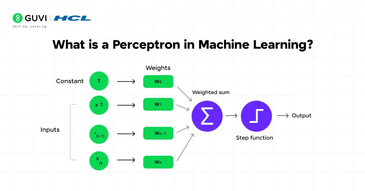
The structure of a perceptron in machine learning includes several key components:
- Inputs: Values representing features or properties of the data
- Weights: Numbers that indicate the importance of each input
- Bias: An additional parameter that helps adjust the output
- Weighted sum: The combined inputs multiplied by their respective weights
- Activation function: Typically a step function that converts the weighted sum into a binary output
The perceptron operates by taking numerical inputs, multiplying them by weights, summing the products with the bias, and passing the sum through an activation function to produce a final classification output.
Why it matters in machine learning
The significance of perceptrons extends beyond their simple structure. As the simplest form of a neural network, perceptrons laid the groundwork for more advanced AI systems we use today.
Despite being developed over 60 years ago, the perceptron algorithm remains fundamental to how we train deep networks today. This model proved that machines could learn to recognize patterns and make predictions based on data, establishing the foundation for supervised learning techniques.
Furthermore, perceptrons demonstrated the possibility of creating computational systems that could adapt and improve over time. By adjusting weights through training, these models introduced the concept of machine learning as we understand it today.
Launch your AI career with HCL GUVI’s Artificial Intelligence and Machine Learning Course. Learn ML, Deep Learning, LLMs, RAG, and AI Agents through live classes, hands-on projects, expert mentorship, and an industry-recognized certification—plus placement assistance to help you land top AI/ML roles. Enroll today and transform your potential into a future-ready AI career.
How a Perceptron Works: Step-by-Step
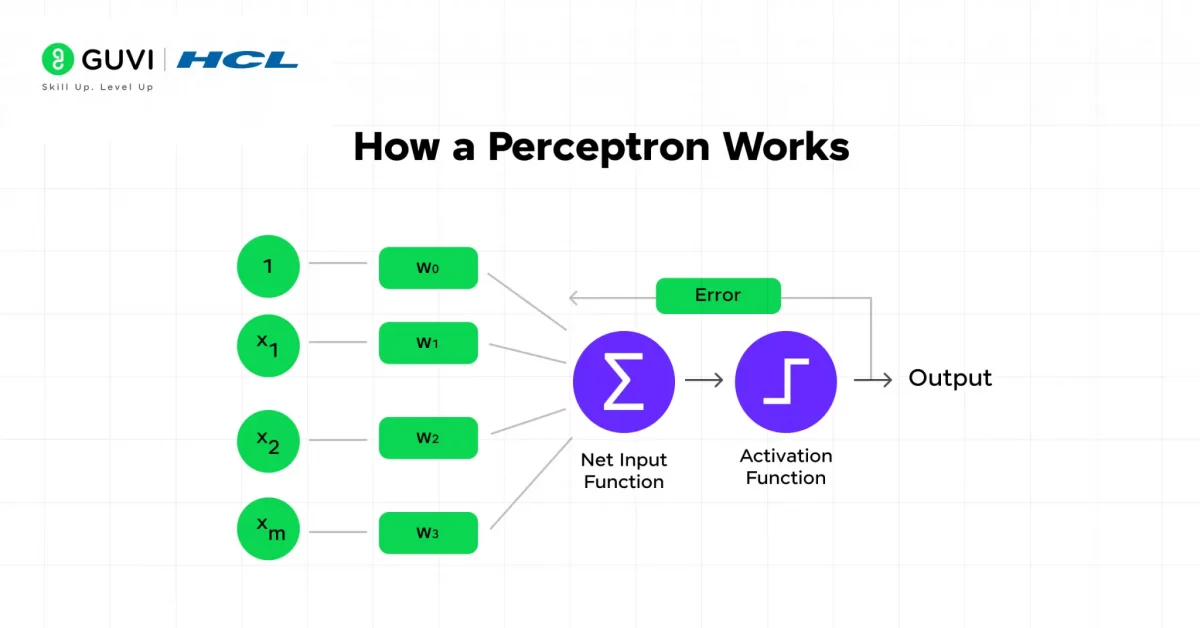
Understanding how a perceptron in machine learning works requires breaking down its computational process into simple, sequential steps. The perceptron model in machine learning processes information through four key stages that transform raw inputs into meaningful classifications.
1) Inputs, weights, and bias
Every perceptron in machine learning begins with three fundamental components that drive its decision-making process:
- Inputs: These are the numerical values that represent features of the data being analyzed. In a perceptron, inputs can be binary (0 or 1) or continuous real numbers. For instance, if you’re building a perceptron to classify emails, inputs might represent features like word frequency or message length.
- Weights: Each input is assigned a specific weight that signifies its importance in the decision-making process. Higher weights indicate a stronger influence on the output. Initially, these weights might be randomly assigned, but they get adjusted during training.
- Bias: This additional parameter shifts the decision boundary away from the origin. The bias acts as another tunable parameter that improves the model’s performance even when all inputs are zero. Think of bias as the perceptron’s baseline tendency to output a particular result.
2) Calculating the weighted sum
Once you have the inputs and weights ready, the next step involves computing their weighted sum:
- Multiply each input by its corresponding weight
- Add all these products together
- Add the bias term to this sum
This calculation can be expressed mathematically as: Weighted sum = (x₁ × w₁) + (x₂ × w₂) + … + (xₙ × wₙ) + b
Where x represents inputs, w represents weights, and b is the bias. This weighted sum gives an appropriate representation of the inputs based on their relative importance.
3) Applying the activation function
Subsequently, the perceptron in machine learning passes this weighted sum through an activation function, introducing non-linearity to the output. Several activation functions can be used, including:
- Heavisine step function: The most common for basic perceptrons, outputting 1 if the weighted sum exceeds the threshold and 0 otherwise
- Sign function: Similar to the step function, but outputs either +1 or -1
- Sigmoid function: Outputs values between 0 and 1, useful for probability-based outputs
The activation function essentially determines whether the perceptron in machine learning will “fire” (activate) based on the calculated value. For the Heavisine step function:
if weighted_sum >= threshold:
output = 1
else:
output = 0
4) Generating the output
The final stage produces the perceptron’s decision or prediction based on the activation function’s result. In the simplest form, the output is binary (0 or 1), representing classifications such as:
- Yes/No decisions
- True/False classifications
- Belong/Don’t belong to a category
For binary classification problems, this output represents the perceptron’s decision about which class the input belongs to. The perceptron model attempts to separate positive and negative classes by learning the optimal values for weights and bias.
During training, the weights and bias are adjusted to minimize errors, but for prediction (after training is complete), the process simply flows through these four steps to generate an output.
The beauty of the perceptron in machine learning lies in its simplicity – just four straightforward steps transform numerical inputs into meaningful classifications, forming the foundation for more complex neural networks in machine learning.
Perceptron vs Logistic Regression: The Mathematical Difference
If you’re learning about a perceptron in machine learning, you’ve probably wondered how it’s different from logistic regression — since both look almost identical on the surface. Both take inputs, multiply them by weights, add a bias, and produce an output. But the way they make decisions is where things actually split apart, and understanding this difference is key to really getting how a perceptron in machine learning works.
Here’s the simplest way to think about it:
- A perceptron makes a hard decision. It looks at the weighted sum and says “yes” or “no” — output is either 0 or 1, nothing in between.
- Logistic regression makes a soft decision. Instead of a flat yes/no, it gives you a probability, like “there’s a 78% chance this is a yes.”
- The perceptron uses a step function (a simple on/off switch), while logistic regression uses a sigmoid function (a smooth S-shaped curve).
- Because of this, logistic regression can tell you how confident it is. A perceptron can’t — it just picks a side.
Example: Imagine you’re classifying emails as spam or not spam.
- A perceptron will simply say: “Spam” or “Not Spam.”
- Logistic regression will say: “This is 92% likely to be spam” — giving you room to set your own confidence threshold.
Here’s a quick difference table:
| Feature | Perceptron | Logistic Regression |
|---|---|---|
| Output type | Binary (0 or 1) | Probability (0 to 1) |
| Activation function | Step function | Sigmoid function |
| Decision style | Hard boundary | Soft, probabilistic boundary |
| Sensitive to outliers | Yes, quite a bit | Less sensitive |
At the end of the day, a perceptron in machine learning is more like a strict yes/no gatekeeper, while logistic regression is more like an advisor giving you odds. Both are foundational, but logistic regression’s probability-based approach is why it’s still widely used today, even outside of neural networks.
Types of Perceptron Models
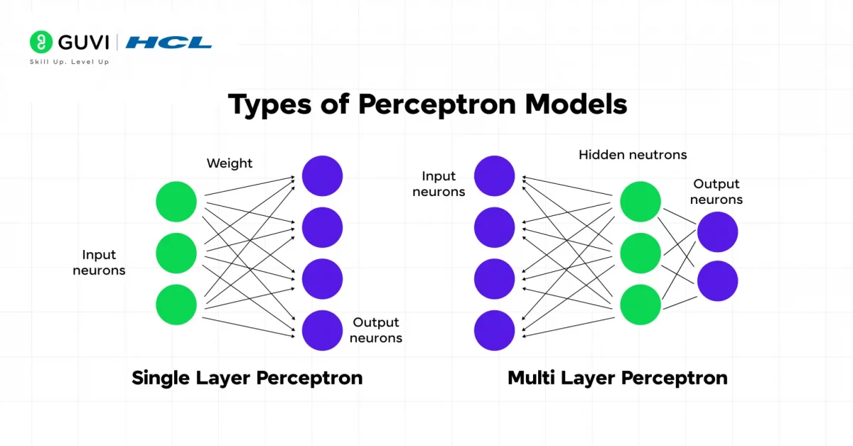
Perceptron models in machine learning come in different varieties, each with distinct capabilities and applications. First of all, let’s explore the two main types of perceptron architectures that form the foundation of neural network development.
1) Single-layer perceptron: basics and use cases
The single-layer perceptron in machine learning (SLP) represents the original and most basic form of neural network, first introduced by Frank Rosenblatt in 1958. This foundational model consists of just an input layer directly connected to an output layer with no hidden layers between them.
How an SLP works:
- Takes inputs from the input layer
- Applies weights to these inputs and sums them
- Passes this sum through an activation function to produce output
A single-layer perceptron in machine learning is particularly effective for tasks involving linearly separable data – situations where a straight line can cleanly divide input data into distinct categories. Primarily, SLPs excel at computing logical operations such as AND, OR, and NOR gates with binary inputs and outputs.
The original perceptron in machine learning used a step function that produced only 0 or 1 as output, whereas modern implementations often use sigmoid activation functions because they’re smoother and work better with gradient-based learning methods.
2) Multi-layer perceptron: structure and power
In contrast, a multi-layer perceptron (MLP) contains one or more hidden layers positioned between the input and output layers. This more advanced architecture forms the basis of deep learning and can handle data that isn’t linearly separable.
The structure of an MLP includes:
- An input layer that receives data
- One or more hidden layers with neurons using nonlinear activation functions
- An output layer that produces predictions
MLPs evolved specifically to overcome the limitations of single-layer perceptrons. Notably, they function as universal approximators, meaning they can model virtually any continuous function with sufficient neurons in their hidden layers. This capability makes them extraordinarily versatile for complex pattern recognition tasks.
Each layer in an MLP connects fully to the next layer, creating a dense network of interconnections that enables the processing of intricate relationships within data. Additionally, MLPs use continuous activation functions such as sigmoid or ReLU rather than step functions, enabling more nuanced outputs and more efficient learning.
Training a Perceptron: Learning Algorithm Explained
The perceptron learning algorithm enables machine learning models to improve through experience. This supervised learning method teaches perceptrons how to classify data by adjusting their weights based on errors.
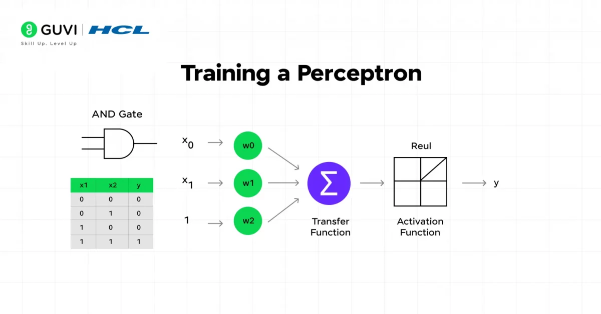
A) What is the perceptron learning rule?
The perceptron learning rule is a supervised training algorithm that adjusts weights and bias to minimize classification errors. It forms the foundation of neural networks by allowing perceptrons to learn from labeled examples.
Primarily, this rule works by:
- Comparing the perceptron’s output with the correct target value
- Calculating the error between the prediction and the actual value
- Adjusting weights and bias accordingly to reduce errors
This learning process follows a forward propagation step (making predictions) followed by backward propagation (adjusting weights based on errors).
B) Perceptron learning algorithm example
Let’s examine the AND gate problem as a simple example. For this binary classification task:

- Start with random weights (e.g., w₁ = 0.9, w₂ = 0.9) and set a learning rate (0.5)
- For input (0,0):
- Weighted sum = (0×0.9) + (0×0.9) = 0
- Activation output = 0 (correct, no weight update needed)
- For input (0,1):
- Weighted sum = (0×0.9) + (1×0.9) = 0.9
- Activation output = 1 (incorrect, should be 0)
- Update weights: w₁ = 0.9 – 0.5 = 0.4, w₂ = 0.9 – 0.5 = 0.4
The algorithm continues through all training examples, adjusting weights whenever a misclassification occurs.
C) How weights and bias are updated
The mathematical formula for updating weights is:
w_new = w_old + η(y – ŷ)x
Where:
- w_old is the current weight
- η (eta) is the learning rate
- y is the actual target value
- ŷ is the predicted output
- x is the input value
Similarly, the bias is updated using:
b_new = b_old + η(y – ŷ)
The error term (y – ŷ) determines both the direction and magnitude of weight adjustments. When the prediction matches the target (y = ŷ), no update occurs.
D) Convergence and stopping criteria
The perceptron learning algorithm will converge if the data is linearly separable, meaning a hyperplane exists that can perfectly separate the classes. Accordingly, the algorithm continues until:
- All training examples are correctly classified, or
- A maximum number of iterations (epochs) is reached
The Perceptron Convergence Theorem guarantees that for linearly separable data, the algorithm will find a solution after a finite number of iterations.
The learning rate significantly influences convergence speed. A large learning rate helps the model learn faster but might reduce accuracy, whereas a smaller learning rate improves accuracy but requires more training time. Typical practice involves testing learning rates on a logarithmic scale between very small values (like 0.0001) and 1.0.
The perceptron might seem simple today, but it was revolutionary when introduced!
Birth of the Perceptron (1957): Frank Rosenblatt developed the perceptron at Cornell University, and the U.S. Navy even funded his work, calling it a step toward “thinking machines.”
Hardware Implementation: Unlike today’s software models, the first perceptron was actually built as a physical machine called the Mark I Perceptron, using motors and electronic circuits to simulate a neural network.
Media Buzz: In the late 1950s, newspapers hailed the perceptron as a breakthrough that could “walk, talk, see, write, reproduce itself and be conscious of its existence” — a reminder of how hyped AI was even back then!
These little stories show how the perceptron not only shaped the history of AI but also captured the public imagination long before deep learning existed.
Building a Simple Perceptron from Scratch in Python (No Sklearn)
The best way to truly understand a perceptron in machine learning is to build one yourself, without relying on any library to do the thinking for you. It’s simpler than it sounds — just a few lines of Python, and you’ll see exactly how a perceptron learns from data.
We’ll build it in four steps: initialize the weights, calculate the output, define the learning rule, and train it on a simple example.
Step 1: Initialize weights and bias
import numpy as np

class Perceptron:
    def __init__(self, input_size, learning_rate=0.1, epochs=10):
        self.weights = np.zeros(input_size)
        self.bias = 0
        self.lr = learning_rate
        self.epochs = epochs
Step 2: Define the activation function
This is what makes a perceptron in machine learning a “hard” classifier — it simply checks if the weighted sum crosses zero.
def activation(self, x):
        return 1 if x >= 0 else 0
Step 3: Calculate the weighted sum and predict
def predict(self, inputs):
        weighted_sum = np.dot(inputs, self.weights) + self.bias
        return self.activation(weighted_sum)
Step 4: Train the perceptron using the learning rule
This is where the model actually learns — adjusting weights whenever it makes a mistake.
def fit(self, X, y):
        for epoch in range(self.epochs):
            for inputs, label in zip(X, y):
                prediction = self.predict(inputs)
                error = label - prediction
                self.weights += self.lr * error * inputs
                self.bias += self.lr * error
Putting it all together — training on the AND gate
A simple AND logic gate is a perfect first example, since it’s linearly separable and shows exactly how a perceptron in machine learning solves basic classification problems.
X = np.array([[0,0], [0,1], [1,0], [1,1]])
y = np.array([0, 0, 0, 1])

model = Perceptron(input_size=2)
model.fit(X, y)

for inputs in X:
    print(inputs, "->", model.predict(inputs))
Output:
[0 0] -> 0
[0 1] -> 0
[1 0] -> 0
[1 1] -> 1
Here’s the full section, polished and restructured:
Limitations and the Path to Deep Learning
Despite being a genuine breakthrough, the perceptron in machine learning wasn’t perfect — and its limitations actually slowed down neural network research for almost two decades. Understanding these limitations isn’t just history trivia; it’s the key to understanding why deep learning exists at all.
1) The linear separability problem
A single-layer perceptron can only solve problems that are linearly separable — meaning you can draw one straight line (or flat plane, in higher dimensions) to cleanly separate the two classes of data.
That sounds fine in theory, but a lot of real-world data just isn’t that neat. Think of it like trying to separate oil and water with a straight stick — no matter how you angle it, some patterns simply can’t be split with a straight line. And when that’s the case, a basic perceptron model has no way to solve it, no matter how long you train it.
2) Why a Single Perceptron Fails: The XOR Problem Explained
The clearest example of this limitation is the XOR (exclusive OR) problem. Here’s the truth table:
| Input A | Input B | Output |
|---|---|---|
| 0 | 0 | 0 |
| 0 | 1 | 1 |
| 1 | 0 | 1 |
| 1 | 1 | 0 |
If you try to plot these points, you’ll notice something interesting: there’s no single straight line that can separate the 1s from the 0s. The pattern needs a curved or bent decision boundary — something a single perceptron in machine learning simply isn’t built to create.
This wasn’t just a footnote in AI history either. In 1969, Marvin Minsky and Seymour Papert highlighted this exact flaw in their book Perceptrons, and it hit the field hard. Funding dried up, interest faded, and it triggered what’s now known as the first “AI winter.”
3) How multi-layer perceptrons solved it
The fix came from a simple but powerful idea: add hidden layers between the input and output.
By stacking layers, multi-layer perceptrons (MLPs) transform the input data into a new space — one where problems like XOR actually become linearly separable. In other words, the hidden layer does the heavy lifting of reshaping the data, so the final layer can draw a clean line through it.
This one shift changed everything:
- MLPs could now create complex, non-linear decision boundaries
- They could approximate almost any continuous function, not just simple linear patterns
- It reignited interest in neural networks, eventually paving the way to the deep learning models we use today
So while the humble perceptron in machine learning couldn’t solve XOR on its own, its limitations directly led to the innovation that built modern AI.
Perceptron vs Neural Network vs Deep Learning: The Evolution Compared
These three terms often get used interchangeably, but they’re really stages of the same idea evolving over time — perceptron first, then neural networks, then deep learning.
| Aspect | Perceptron | Neural Network | Deep Learning |
|---|---|---|---|
| Structure | Single unit, no hidden layers | Multiple layers, usually 1-2 hidden layers | Many hidden layers (often dozens or hundreds) |
| Output type | Binary (0 or 1) | Can be binary, multi-class, or continuous | Can handle highly complex outputs (images, text, speech) |
| Can solve non-linear problems? | No — fails on problems like XOR | Yes, with at least one hidden layer | Yes, and can model extremely complex, high-dimensional patterns |
| Training method | Simple weight-update rule | Backpropagation + gradient descent | Backpropagation + gradient descent (with more advanced optimizers) |
| Data requirement | Small datasets are fine | Moderate datasets | Usually needs large datasets to perform well |
| Compute cost | Very low | Low to moderate | High — often needs GPUs/TPUs |
| Real-world use today | Rarely used alone; mostly educational | Used for simpler, structured problems | Used for image recognition, NLP, speech, self-driving, etc. |
Conclusion
The perceptron in machine learning stands as a fundamental milestone in machine learning history. Through this guide, you’ve learned how this simple computational model mimics biological neurons to make binary classifications based on weighted inputs. Despite being developed over 60 years ago, perceptrons remain remarkably relevant to understanding today’s complex AI systems.
Understanding perceptrons gives you a solid foundation before diving into more advanced neural network architectures. The concepts of inputs, weights, activation functions, and learning algorithms remain consistent throughout neural network theory, though they grow increasingly complex.
I hope this guide helps you begin your learning journey into perceptrons and do reach out to me in the comments section below if you have any doubts. Good Luck!
FAQs
Q1. What is a perceptron in machine learning?
A perceptron is a simple algorithm in machine learning that mimics how biological neurons process information. It’s designed for binary classification tasks, such as determining whether an email is spam or not, by using weighted inputs to make decisions.
Q2. How does a perceptron work?
A perceptron works by taking numerical inputs, multiplying them with assigned weights, summing these products along with a bias, and then passing this sum through an activation function to generate a binary output (typically 0 or 1).
Q3. What are the limitations of a single-layer perceptron?
Single-layer perceptrons can only solve linearly separable problems, meaning they can only classify data that can be separated by a straight line. They cannot handle complex, non-linear problems like the XOR problem.
Q4. How do multi-layer perceptrons differ from single-layer perceptrons?
Multi-layer perceptrons (MLPs) have one or more hidden layers between the input and output layers, allowing them to solve non-linear problems. They can approximate virtually any continuous function, making them more versatile for complex pattern recognition tasks.
Q5. What is the perceptron learning rule?
The perceptron learning rule is a supervised training algorithm that adjusts the weights and bias of a perceptron to minimize classification errors. It compares the perceptron’s output with the correct target value, calculates the error, and adjusts the parameters accordingly to improve performance over time.
Success Stories









Did you enjoy this article?