


Data Science Articles
Accountant vs Data Analyst Salary in India After Switching Careers - Best Guide
Finance Managers: Could Data Science Be Your Next Career Move?
Insurance Claims Executive to Data Analyst: Is It a Good Switch?
Banking Executive (Loans, KYC) to Data Analyst: Skills and Career Path


Get In Touch For Details! Request More Information

What is a Decision Tree in Machine Learning – A Step-by-Step Guide
Sep 19, 2026 10 Min Read 9580 Views
(Last Updated)
Decision trees are one of the most interpretable machine learning algorithms because they turn predictions into a sequence of clear decision rules. Instead of behaving like a black box, a decision tree shows how features are evaluated, where the data is split, and how the final prediction is reached.
A decision tree in machine learning can solve both classification and regression problems. It recursively divides data using criteria such as Gini impurity, information gain, or variance reduction until it reaches leaf nodes containing the final prediction.
This guide explains how decision trees work, how they are built and pruned, the major decision tree algorithms, performance evaluation techniques, advantages and limitations, and practical ways to tune and implement them effectively.
Table of contents
- Quick Answer
- What are Decision Trees?
- What is a Decision Tree in Machine Learning - A Step-by-Step Guide
- How Decision Trees Work
- Building a Decision Tree
- Pruning Decision Trees
- Evaluating Decision Tree Performance
- Advantages and Disadvantages of Decision Trees
- Advantages
- Disadvantages
- Quick Summary
- Decision Tree Algorithms
- a) ID3 (Iterative Dichotomiser 3)
- b) C4.5
- c) CART (Classification and Regression Trees)
- d) CHAID (Chi-Square Automatic Interaction Detection)
- e) Conditional Inference Trees
- Quick Comparison of Decision Tree Algorithms
- Decision Tree Hyperparameters and How to Tune Them
- Example
- How to Tune a Decision Tree
- Decision Tree vs Random Forest vs Gradient Boosting
- When to Use a Decision Tree
- When to Use Random Forest
- When to Use Gradient Boosting
- How to Build a Decision Tree in Python Using Scikit-Learn
- Step 1: Import the Required Libraries
- Step 2: Load and Split the Dataset
- Step 3: Create the Decision Tree Model
- Step 4: Train the Model
- Step 5: Make Predictions
- Step 6: Evaluate Accuracy
- Real-World Applications of Decision Trees in Machine Learning
- Conclusion
- FAQs
- What are the key advantages of using decision trees in machine learning?
- How do decision trees handle missing values in the dataset?
- What are some common techniques to prevent overfitting in decision trees?
Quick Answer
A decision tree is a supervised machine learning algorithm that makes predictions by repeatedly splitting data according to feature-based decision rules.
- Main Structure: Root node, internal decision nodes, branches, and leaf nodes.
- Used For: Both classification and regression problems.
- Split Criteria: Gini impurity, information gain, entropy, and variance reduction.
- Main Strength: Easy to interpret because predictions can be traced through explicit rules.
- Main Limitation: Deep trees can overfit training data unless depth, pruning, and other parameters are controlled.
What are Decision Trees?
Decision trees are flowchart-like structures that model decisions and their possible consequences. They start with a single node (the root) and branch out into possible outcomes, ultimately leading to a final decision or prediction (the leaves).
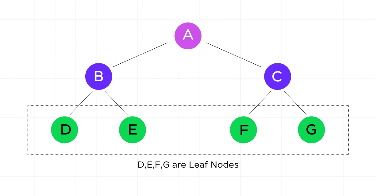
The basic structure of a decision tree includes:
- Root Node: The topmost node, representing the entire dataset.
- Internal Nodes: Decision points where the data is split based on certain conditions.
- Branches: The outcomes of a decision, connecting nodes.
- Leaf Nodes: Terminal nodes that represent the final output or decision.
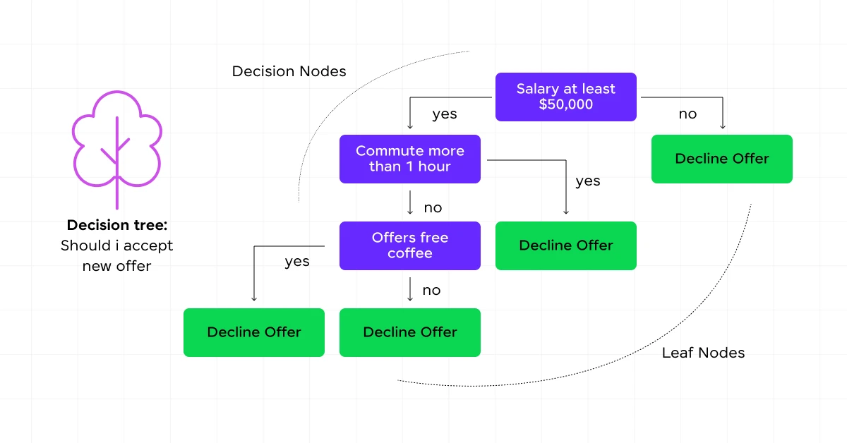
Now, let’s explore how decision trees are used in machine learning with a step-by-step guide.
What is a Decision Tree in Machine Learning – A Step-by-Step Guide
Let’s explore how they work, and how to build and optimize them.
How Decision Trees Work
Decision trees work by recursively splitting the dataset into subsets based on the most significant attribute at each node. The goal is to create homogeneous subsets with respect to the target variable. This process continues until a stopping criterion is met, such as reaching a maximum depth or having a minimum number of samples in a leaf node.
For classification tasks, the decision tree predicts the class label of a new instance by traversing from the root to a leaf node, following the path determined by the decision rules at each internal node. For regression tasks, the prediction is typically the average target value of the training instances that reach a particular leaf node.
The key to understanding how decision trees work lies in grasping the concept of information gain and entropy (for classification) or variance reduction (for regression). These metrics guide the tree-building process by determining the best splits at each node.
Building a Decision Tree
Building a decision tree involves several steps:
a) Feature Selection
Choose the most important feature to split the data at each node. This is typically done using metrics like:
- Information Gain: Measures the reduction in entropy after a dataset is split on an attribute.
- Gini Impurity: Measures the probability of incorrectly classifying a randomly chosen element.
- Variance Reduction: Used for regression trees to minimize the variance in the target variable.
b) Splitting
Once the best feature is selected, the data is split into subsets. For categorical features, this might involve creating a branch for each category. For continuous features, a threshold is chosen to create binary splits.
c) Recursive Partitioning
Steps a and b are repeated recursively for each subset until a stopping criterion is met.
d) Assigning Leaf Nodes
Once splitting stops, the majority class (for classification) or average value (for regression) of the remaining instances is assigned to the leaf node.
The process of building a decision tree aims to maximize the homogeneity of the target variable within each subset. This is achieved by choosing splits that result in the highest information gain or the largest reduction in impurity.
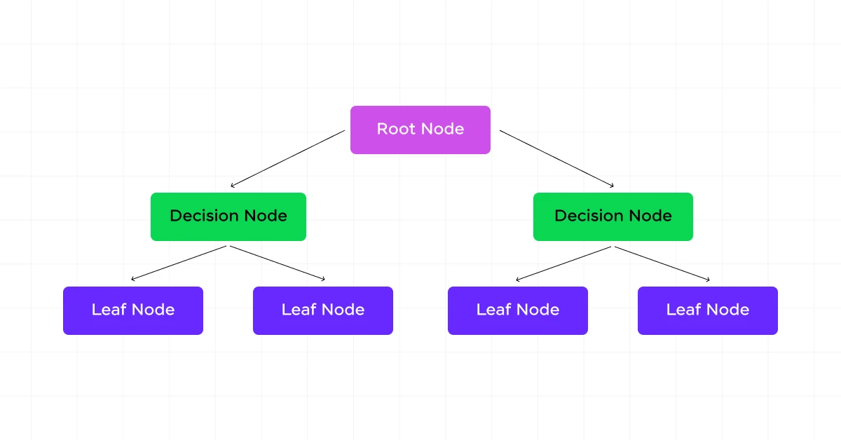
Let’s consider a simple example: Suppose we’re building a decision tree to predict whether a customer will purchase a product based on their age and income. We start with the root node containing all customers. We then evaluate which feature (age or income) provides the best split. Let’s say income gives the highest information gain.
We create two branches: one for “income <= Rs. 50,000” and another for “income > Rs. 50,000”. We then repeat this process for each of these new nodes, possibly splitting on age next. This continues until we reach our stopping criteria.
Pruning Decision Trees
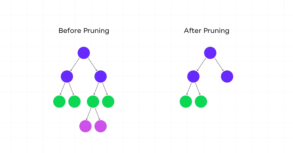
While decision trees are powerful, they can easily overfit the training data, leading to poor generalization on unseen data. Pruning is a technique used to reduce the size of decision trees by removing sections of the tree that provide little power to classify instances.
There are two main approaches to pruning:
a) Pre-pruning (Early Stopping)
- Set constraints before tree construction begins.
- Examples include setting a maximum tree depth, a minimum number of samples required to split an internal node, or a minimum number of samples required to be at a leaf node.
- While computationally efficient, it can be challenging to choose the right parameters without prior knowledge.
b) Post-pruning
- Build the full tree first, then remove branches that don’t provide significant predictive power.
- Common methods include:
- Reduced Error Pruning: Replace each node with its most popular class. If the prediction accuracy doesn’t decrease, keep it pruned.
- Cost Complexity Pruning: Balance between tree size and misclassification rate using a complexity parameter.
Pruning helps to combat overfitting by reducing the complexity of the final classifier, which often improves predictive accuracy on unseen data. It’s an important step in the decision tree-building process, especially when dealing with noisy or limited data.
You must also go through the Top 9 Machine Learning Project Ideas For All Levels [with Source Code].
Evaluating Decision Tree Performance
Evaluating the performance of a decision tree model is important to understand its effectiveness and to compare it with other models. Several metrics and techniques are commonly used:
a) Accuracy: The proportion of correct predictions (both true positives and true negatives) among the total number of cases examined. While intuitive, accuracy can be misleading for imbalanced datasets.
b) Precision and Recall: Precision is the ratio of true positives to all positive predictions, while recall (also known as sensitivity) is the ratio of true positives to all actual positive cases. These metrics are particularly useful when class imbalance is present.
c) F1 Score: The harmonic mean of precision and recall, providing a single score that balances both metrics.
d) Confusion Matrix: A table that describes the performance of a classification model by showing the counts of true positives, true negatives, false positives, and false negatives.
e) ROC Curve and AUC: The Receiver Operating Characteristic (ROC) curve plots the true positive rate against the false positive rate at various threshold settings. The Area Under the Curve (AUC) provides an aggregate measure of performance across all possible classification thresholds.
f) Mean Squared Error (MSE) or Mean Absolute Error (MAE): For regression trees, these metrics measure the average squared or absolute differences between predicted and actual values.
g) Cross-validation: A technique to assess how the results of a statistical analysis will generalize to an independent dataset. It’s particularly useful for evaluating how well a decision tree model will perform on unseen data.
When evaluating decision trees, it’s important to consider not just the overall performance metrics, but also the tree’s interpretability and complexity. A slightly less accurate but more interpretable tree might be preferred in some applications where understanding the decision-making process is important.
Advantages and Disadvantages of Decision Trees
Like any machine learning algorithm, decision trees offer clear benefits but also have limitations that affect model accuracy, stability, and scalability. Understanding these trade-offs helps determine when a decision tree is the right model and when an ensemble method may work better.
Advantages
1. Easy to Interpret
Decision trees represent predictions as a sequence of human-readable rules.
For example:
Age < 30 → Income > ₹50,000 → Likely to Purchase
This makes it easier to explain why a model produced a specific prediction compared with many black-box models.
2. Works With Numerical and Encoded Categorical Features
Decision trees can split numerical features using thresholds such as:
Income <= 50000
Categorical features can also be used after suitable encoding when the implementation requires numerical input. Some tree algorithms support categorical variables directly, while libraries such as Scikit-learn typically expect encoded feature values.
3. No Assumption About Data Distribution
Decision trees are non-parametric models. They do not require the input data to follow a normal, linear, or other predefined statistical distribution.
This makes them useful when relationships between features and the target are nonlinear or irregular.
4. Captures Nonlinear Relationships
Decision trees can model complex feature interactions without manually creating interaction terms.
For example, customer churn might depend on:
Contract Type → Monthly Charges → Support Calls
The tree can learn this sequence directly from the data.
5. Provides Feature Importance
Decision tree models can estimate how much each feature contributes to reducing impurity across the tree.
This helps identify which variables influence predictions most strongly.
However, feature importance should not automatically be interpreted as causality.
6. Minimal Feature Scaling Requirements
Decision trees generally do not require normalization or standardization because splits are based on feature thresholds rather than distance calculations.
For example, a model can directly compare:
- Age = 25
- Salary = ₹80,000
- Number of purchases = 12
without scaling these values to a common range.
This reduces the amount of data preparation required compared with algorithms such as K-Means, KNN, or SVM.
7. Supports Both Classification and Regression
The same tree-based structure can solve different prediction problems.
- Classification Tree: Predicts classes such as fraud or legitimate.
- Regression Tree: Predicts numerical values such as house price or demand.
8. Can Handle Feature Interactions Automatically
Decision trees naturally learn combinations of conditions.
For example:
Credit Score > 700 AND Debt Ratio < 30%
may lead to a different prediction than either feature alone.
This reduces the need to manually engineer interaction terms.
Disadvantages
1. High Risk of Overfitting
An unrestricted decision tree can keep splitting until it memorizes the training data.
For example, a very deep tree may produce:
- Training accuracy: 100%
- Test accuracy: much lower
This indicates poor generalization.
Common controls include:
max_depthmin_samples_splitmin_samples_leafccp_alpha
2. Sensitive to Small Changes in Data
Decision trees can be unstable.
A small change in the training dataset may change the feature selected at the root node, which can alter the structure of the entire tree.
Ensemble methods such as Random Forest reduce this instability by combining predictions from multiple trees.
3. Can Become Biased With Imbalanced Classes
If 95% of training examples belong to one class, a decision tree may learn splits that favor the majority class.
For imbalanced datasets, consider:
- Class weights
- Resampling
- Precision and recall
- F1-score
- ROC-AUC or PR-AUC where appropriate
Accuracy alone may be misleading.
4. Uses Greedy Split Selection
Most decision tree algorithms choose the best available split at the current node.
They do not normally evaluate every possible complete tree structure before deciding.
As a result, a locally optimal split does not guarantee a globally optimal final tree.
5. Deep Trees Become Hard to Interpret
A small tree with five or six levels may be easy to explain.
A tree containing hundreds of nodes becomes difficult to visualize, audit, and maintain.
This weakens one of the main advantages of decision trees: interpretability.
6. Regression Trees Cannot Extrapolate Well
A regression tree predicts values based on the training samples reaching each leaf.
If the training target ranges from ₹20,000 to ₹1,00,000, the tree generally cannot meaningfully predict far beyond that observed range.
This makes decision trees weak at extrapolating trends outside the training data.
7. Axis-Aligned Splits Can Require Large Trees
Standard decision trees usually create one-feature-at-a-time splits such as:
Age <= 35
or:
Income > 60000
If the true decision boundary depends on a diagonal or more complex combination of features, the model may need many splits to approximate it.
8. Feature Importance Can Be Misleading
Impurity-based feature importance can sometimes favor variables with many possible split points.
For more reliable interpretation, techniques such as permutation importance or SHAP can be used alongside the tree’s built-in importance scores.
Quick Summary
| Advantages | Disadvantages |
|---|---|
| Easy to interpret | Can overfit easily |
| Handles nonlinear relationships | Sensitive to small data changes |
| No feature scaling required | Can favor majority classes |
| Supports classification and regression | Greedy splitting may be suboptimal |
| Provides feature importance | Deep trees lose interpretability |
| Captures interactions automatically | Regression trees extrapolate poorly |
| Requires limited preprocessing | Complex boundaries may require many splits |
Decision trees are especially useful when interpretability, rule-based decisions, and fast baseline modelling matter. When stability and predictive performance are more important, ensemble techniques such as Random Forest or gradient boosting are often preferred.
Also Read: Supervised and Unsupervised Learning: Explained with Detailed Categorization
Decision Tree Algorithms
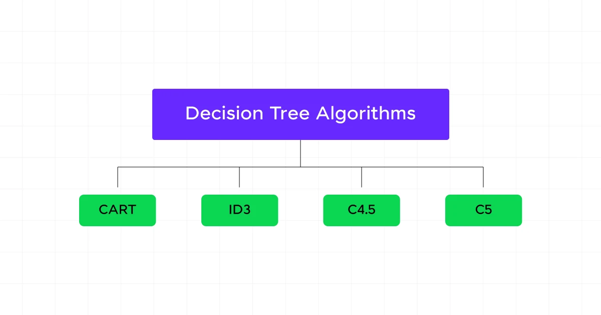
Different decision tree algorithms use different criteria to choose the best feature and threshold at each node. They also differ in whether they support classification, regression, continuous variables, missing values, multiway splits, and pruning.
a) ID3 (Iterative Dichotomiser 3)
ID3 was introduced by Ross Quinlan and is primarily designed for classification problems involving categorical features.
- Splitting Criterion: Uses Information Gain, which measures how much a split reduces entropy.
- Split Selection: Evaluates available attributes and chooses the one producing the highest Information Gain.
- Tree Structure: Can create multiple branches when a categorical feature contains multiple values.
- Target Variable: Designed for categorical class labels.
- Continuous Features: Original ID3 does not directly handle continuous variables without first converting them into categories.
- Missing Values: Has limited native support compared with later algorithms.
- Pruning: Original ID3 does not include post-pruning.
- Main Limitation: Information Gain can favor attributes containing many unique values.
Best suited for: Small classification datasets containing mostly categorical variables.

b) C4.5
C4.5 was developed by Ross Quinlan as an extension of ID3 to overcome several of its limitations.
- Splitting Criterion: Uses Gain Ratio, which adjusts Information Gain to reduce its preference for attributes with many distinct values.
- Continuous Features: Can determine threshold-based splits for numerical variables.
- Categorical Features: Supports discrete attributes and can create appropriate branches for their values.
- Missing Values: Can account for records with unknown attribute values during tree construction.
- Pruning: Uses post-pruning to remove branches that are unlikely to improve performance on unseen data.
- Tree Output: Produces a classification tree and can also convert the final tree into readable decision rules.
- Main Advantage: More practical for real-world datasets than ID3 because it handles continuous features, missing values, and overfitting more effectively.
Best suited for: Classification problems containing a mixture of numerical and categorical features.
c) CART (Classification and Regression Trees)
CART, introduced by Leo Breiman, Jerome Friedman, Richard Olshen, and Charles Stone, supports both classification and regression.
- Classification Criterion: Commonly uses Gini impurity to identify splits that create purer class groups.
- Regression Criterion: Uses reduction in prediction error, commonly based on squared error, to divide numerical targets.
- Tree Structure: CART always creates binary splits, meaning every internal node has exactly two child branches.
- Classification Output: Leaf nodes predict a class or class probability.
- Regression Output: Leaf nodes predict a numerical value, typically derived from training samples reaching that leaf.
- Pruning: Supports cost-complexity pruning, which balances predictive fit against tree complexity.
- Continuous Features: Tests candidate thresholds such as
age <= 35. - Categorical Data: Practical implementations may require categorical variables to be encoded before training.
CART is especially important in Python because Scikit-learn’s DecisionTreeClassifier and DecisionTreeRegressor follow the CART-style binary tree approach.
Best suited for: General classification and regression problems where binary decision rules and interpretable predictions are required.
d) CHAID (Chi-Square Automatic Interaction Detection)
CHAID constructs decision trees using statistical significance tests rather than impurity measures such as Gini or entropy.
- Splitting Criterion: Uses the chi-square test for categorical target variables to measure the association between predictors and the target.
- Category Merging: Categories that are statistically similar can be combined before the final split is created.
- Tree Structure: Can create more than two branches from a single node.
- Stopping: Tree growth can stop when no statistically significant relationship remains between candidate predictors and the target.
- Strength: Produces highly interpretable segmentation trees.
- Common Applications: Customer segmentation, survey analysis, marketing research, and demographic analysis.
- Limitation: Its reliance on statistical significance can require relatively large sample sizes for stable results.
Best suited for: Segmentation and classification problems involving categorical or discretized variables.
e) Conditional Inference Trees
Conditional Inference Trees use a statistical testing framework to decide whether a split should occur and which variable should be selected.
- Split Selection: Tests the statistical association between each predictor and the response variable.
- Variable Selection: Selects the predictor with the strongest statistically significant association with the target.
- Stopping Rule: Stops splitting when no predictor shows sufficient statistical evidence of association.
- Selection Bias: Reduces the tendency of traditional tree algorithms to prefer variables with many possible split points or categories.
- Pruning: Separate post-pruning is generally unnecessary because statistical hypothesis tests control tree growth during construction.
- Output: Produces interpretable decision rules while controlling unnecessary splits.
- Main Advantage: Separates the decision of whether to split from the decision of where to split.
Best suited for: Statistical modelling problems where unbiased feature selection and interpretable tree structures are important.
Quick Comparison of Decision Tree Algorithms
| Algorithm | Main Split Criterion | Classification | Regression | Continuous Features | Split Type | Pruning/Growth Control |
|---|---|---|---|---|---|---|
| ID3 | Information Gain | Yes | No | Limited | Multiway | No built-in pruning |
| C4.5 | Gain Ratio | Yes | No | Yes | Binary or multiway | Post-pruning |
| CART | Gini / prediction error | Yes | Yes | Yes | Binary only | Cost-complexity pruning |
| CHAID | Chi-square statistical tests | Yes | Limited by implementation | Usually discretized | Multiway | Significance-based stopping |
| Conditional Inference Tree | Statistical hypothesis tests | Yes | Yes | Yes | Typically recursive binary partitions | Statistical stopping |
In practice, CART is one of the most relevant algorithms for Python machine learning, while C4.5 is important for understanding how decision trees evolved beyond ID3. CHAID is especially useful for segmentation, and Conditional Inference Trees are valuable when reducing feature-selection bias is important.
Kickstart your Data Science journey by enrolling in HCL GUVI’s Data Science Course where you will master technologies like MongoDB, Tableau, PowerBI, Pandas, etc., and build interesting real-life projects. Alternatively, if you would like to explore Python through a Self-paced course, try HCL GUVI’s Python course.
Decision Tree Hyperparameters and How to Tune Them
A decision tree can fit training data extremely closely if its growth is not controlled. Hyperparameter tuning determines how deep the tree can grow, when it can split, and how much data must remain in each leaf.
The most important decision tree hyperparameters include:
| Hyperparameter | What It Controls | Practical Effect |
|---|---|---|
max_depth | Maximum number of levels in the tree | Lower values reduce complexity and overfitting |
min_samples_split | Minimum samples required to split an internal node | Larger values prevent tiny, highly specific branches |
min_samples_leaf | Minimum samples allowed in a leaf | Helps produce more stable predictions |
max_features | Number of features considered when finding a split | Can reduce correlation and complexity |
criterion | Metric used to evaluate splits | Common options include Gini and entropy for classification |
ccp_alpha | Cost-complexity pruning strength | Larger values prune more branches |
Example
Suppose a fully grown classification tree reaches a training accuracy of 100% but performs poorly on validation data.
Instead of keeping the unrestricted model, you might test:
DecisionTreeClassifier(
    max_depth=5,
    min_samples_split=10,
    min_samples_leaf=5,
    random_state=42
)
This prevents the tree from creating branches based on very small groups of training examples.
How to Tune a Decision Tree
A practical tuning process is:
- Split the dataset into training and validation sets.
- Train a simple baseline tree.
- Check training and validation performance.
- Test different values for depth and minimum samples.
- Use cross-validation to compare configurations.
- Select the simplest tree that maintains acceptable validation performance.
The goal is not to build the deepest possible decision tree. It is to find enough complexity to capture useful patterns without memorizing the training dataset.
Decision Tree vs Random Forest vs Gradient Boosting
Decision trees form the foundation of several powerful ensemble machine learning techniques. Random Forest and gradient boosting both use multiple trees, but they combine them differently.
| Factor | Decision Tree | Random Forest | Gradient Boosting |
|---|---|---|---|
| Number of Trees | One | Many | Many |
| Training Style | Single tree | Trees trained largely independently | Trees trained sequentially |
| Interpretability | High | Moderate to low | Lower |
| Overfitting Risk | Relatively high | Lower than single tree | Depends heavily on tuning |
| Prediction | One tree output | Aggregates multiple trees | Combines sequential corrections |
| Main Strength | Simplicity and explainability | Stability and generalization | Strong predictive performance |
| Typical Use | Explainable baseline models | Robust general-purpose models | High-performance structured-data models |
When to Use a Decision Tree
Choose a single decision tree when:
- Interpretability is important.
- You need explicit decision rules.
- The dataset is relatively small or moderate.
- You want a fast baseline model.
- Stakeholders need to understand why predictions are made.
When to Use Random Forest
Random Forest is useful when a single tree is unstable or overfits. It trains multiple trees using different samples and feature subsets, then combines their predictions.
When to Use Gradient Boosting
Gradient boosting is useful when predictive performance is more important than individual-tree interpretability. Each new tree focuses on correcting errors made by earlier trees.
A single decision tree is therefore often the easiest model to explain, while tree ensembles are usually chosen when stronger generalization or predictive performance is required.
How to Build a Decision Tree in Python Using Scikit-Learn
Python’s scikit-learn library provides decision tree models for both classification and regression.
A typical classification workflow includes data preparation, train-test splitting, model training, prediction, and evaluation.
Step 1: Import the Required Libraries
from sklearn.datasets import load_iris
from sklearn.model_selection import train_test_split
from sklearn.tree import DecisionTreeClassifier
from sklearn.metrics import accuracy_score
Step 2: Load and Split the Dataset
data = load_iris()

X = data.data
y = data.target

X_train, X_test, y_train, y_test = train_test_split(
    X,
    y,
    test_size=0.2,
    random_state=42
)
Step 3: Create the Decision Tree Model
model = DecisionTreeClassifier(
    max_depth=4,
    random_state=42
)
Step 4: Train the Model
model.fit(X_train, y_train)
Step 5: Make Predictions
predictions = model.predict(X_test)
Step 6: Evaluate Accuracy
accuracy = accuracy_score(y_test, predictions)

print("Accuracy:", accuracy)
The same general workflow applies to regression, but DecisionTreeRegressor replaces DecisionTreeClassifier, and regression metrics such as MAE or MSE are used instead of classification accuracy.
A production workflow should also include cross-validation, hyperparameter tuning, class imbalance checks where relevant, and evaluation on data that was not used during training.
Real-World Applications of Decision Trees in Machine Learning
Decision trees are useful when predictions need to be both accurate enough for the task and understandable to humans. Their rule-based structure makes them especially useful in applications where the reasoning behind a prediction matters.
- Banking and Credit Risk: Decision trees can classify loan applicants using variables such as income, repayment history, debt levels, and credit-related features.
- Healthcare: Trees can help categorize patient risk using symptoms, test values, demographic variables, or clinical measurements.
- Customer Churn Prediction: Businesses can identify customers at risk of leaving based on usage patterns, transaction history, engagement, and service interactions.
- Fraud Detection: Decision rules can separate normal and potentially suspicious transactions using amounts, locations, frequencies, and behavioural signals.
- Marketing: Decision trees can segment customers based on purchase history, demographics, campaign responses, and engagement.
- Manufacturing: Sensor readings and production variables can be used to classify equipment conditions or predict potential faults.
- Insurance: Decision trees can support risk categorization, claim analysis, and policy-related predictions.
- HR Analytics: Employee data can be analysed to identify patterns associated with attrition, performance, or workforce planning.
Conclusion
A decision tree in machine learning converts complex datasets into structured decision rules that are relatively easy to interpret. By recursively splitting data using criteria such as Gini impurity, information gain, or variance reduction, decision trees can handle both classification and regression problems.
Their simplicity is also their main limitation. An unrestricted tree can become deep, unstable, and overfit the training data. Techniques such as pruning, depth limits, minimum sample constraints, cross-validation, and hyperparameter tuning help improve generalization.
Decision trees also provide the foundation for advanced ensemble methods such as Random Forest and gradient boosting, making them an important concept to understand before moving to more complex machine learning models.
FAQs
What are the key advantages of using decision trees in machine learning?
Decision trees offer several advantages, including:
1. Interpretability: The tree structure is easy to visualize and understand, making it simple to interpret and explain the decision-making process.
2. Handling of Non-Linear Data: Decision trees can capture non-linear relationships between features without requiring extensive data preprocessing.
3. Versatility: They can be used for both classification and regression tasks, making them a flexible tool in a data scientist’s arsenal.
How do decision trees handle missing values in the dataset?
Decision trees have built-in mechanisms to handle missing values. During the tree-building process, if a feature value is missing for a certain sample, the algorithm can:
1. Surrogate Splits: Use surrogate splits, which are alternative splits based on other features that closely mimic the primary split, to make a decision.
2. Imputation: Estimate the missing values based on the most common value or mean of the feature, depending on the type of data.
What are some common techniques to prevent overfitting in decision trees?
Overfitting is a common issue in decision trees, where the model becomes too complex and captures noise rather than the underlying pattern. To prevent overfitting, you can use techniques such as:
1. Pruning: Remove parts of the tree that do not provide significant power to classify instances, either through pre-pruning (setting constraints like maximum depth) or post-pruning (removing nodes after the tree is built).
2. Setting Minimum Split Criteria: Require a minimum number of samples in a node for a split to be considered.
3. Cross-Validation: Use cross-validation to evaluate the model’s performance on different subsets of the data, ensuring it generalizes well to unseen data.
Success Stories

About the Author
Vaishali
I'm a seasoned writer with four years of experience across technical, non-technical, and just about every genre or niche you can imagine. Adaptable and curious, I enjoy exploring new topics and making information engaging and easy to understand. Fueled by a steady stream of tea, I approach each project with creativity, reliability, and genuine enthusiasm for storytelling.
View all posts by Vaishali
Connect with me @














Did you enjoy this article?