


Artificial Intelligence and Machine Learning Articles
Data Analyst vs Machine Learning Engineer: Which Career Grows Faster?
Finance Manager to Data Analytics: Career Growth, Salary and Seniority
How to Evaluate LLM Outputs in Production Deployments
AI/ML Skills Gap 2026: Why Companies Can't Find Job-Ready Talent


Get In Touch For Details! Request More Information
Implementing Agglomerative Clustering using Sklearn
Nov 20, 2026 5 Min Read 1970 Views
(Last Updated)
Agglomerative clustering groups unlabeled data by treating every observation as its own cluster and joining the most similar ones step by step. The result is a hierarchy of nested groups instead of a single flat split.
This makes agglomerative clustering useful when the number of natural groups is unknown, and the relationships between them matter as much as the groups themselves.
Table of contents
- TL;DR
- What is Agglomerative Clustering?
- Understanding Hierarchical Clustering
- Agglomerative Hierarchical Clustering
- Divisive Hierarchical Clustering
- How Bottom-Up Clustering Works
- How Cluster Merging Happens in Agglomerative Clustering
- Types of Linkage Methods
- Ward Linkage
- Complete Linkage
- Single Linkage
- Average Linkage
- Comparison of Linkage Methods in Agglomerative Clustering
- What is a Distance Matrix?
- What is a Dendrogram?
- Implementing Agglomerative Clustering using Sklearn
- Step 1: Import the Required Libraries
- Step 2: Create a Sample Dataset
- Step 3: Apply Agglomerative Clustering
- Step 4: Visualize the Clusters
- Visualizing Clusters using a SciPy Dendrogram
- Step 1: Import SciPy Libraries
- Step 2: Create the Linkage Matrix
- Step 3: Plot the Dendrogram
- How to Choose the Number of Clusters in Agglomerative Clustering
- Cut the Dendrogram
- Set a Distance Threshold
- Use the Silhouette Score
- Advantages of Agglomerative Clustering
- Limitations of Agglomerative Clustering
- Real-World Applications of Agglomerative Clustering
- Conclusion
- FAQs
- What is agglomerative clustering?
- What is the difference between agglomerative and divisive clustering?
- What is the difference between K-means and agglomerative clustering?
- How do you choose the number of clusters in agglomerative clustering?
- What is the time complexity of agglomerative clustering?
TL;DR
- Agglomerative clustering works bottom-up, starting with each point alone and merging the closest clusters until a stopping condition is reached.
- The linkage method sets how cluster distance is measured, and Ward, the sklearn default, favors compact groups of similar size.
- A dendrogram records every merge and its distance, and cutting it at a chosen height yields the final clusters.
- Since no centroids are involved, results stay stable across runs, and a distance threshold removes the need to fix the cluster count in advance.
- Memory and time grow quickly with dataset size; merges cannot be undone, and sklearn has no predict method for new samples.
What is Agglomerative Clustering?
Agglomerative clustering is a hierarchical clustering method used for unsupervised tasks. It starts with each data point as an individual cluster. The algorithm continuously merges clusters until all points belong to one cluster or a certain condition is met.
Because it builds from smaller to larger clusters, it is often called bottom-up clustering.
Unlike k-means clustering, agglomerative clustering does not need to set cluster centers. Instead, it relies on distance measurements and linkage methods to determine how clusters merge.
Spotting hidden structure in raw data is a skill worth owning. If clustering has sparked your curiosity, take the next step with HCL GUVI’s Intel & IITM Pravartak Certified AI/ML Course and learn to turn patterns into real, working projects.
Understanding Hierarchical Clustering
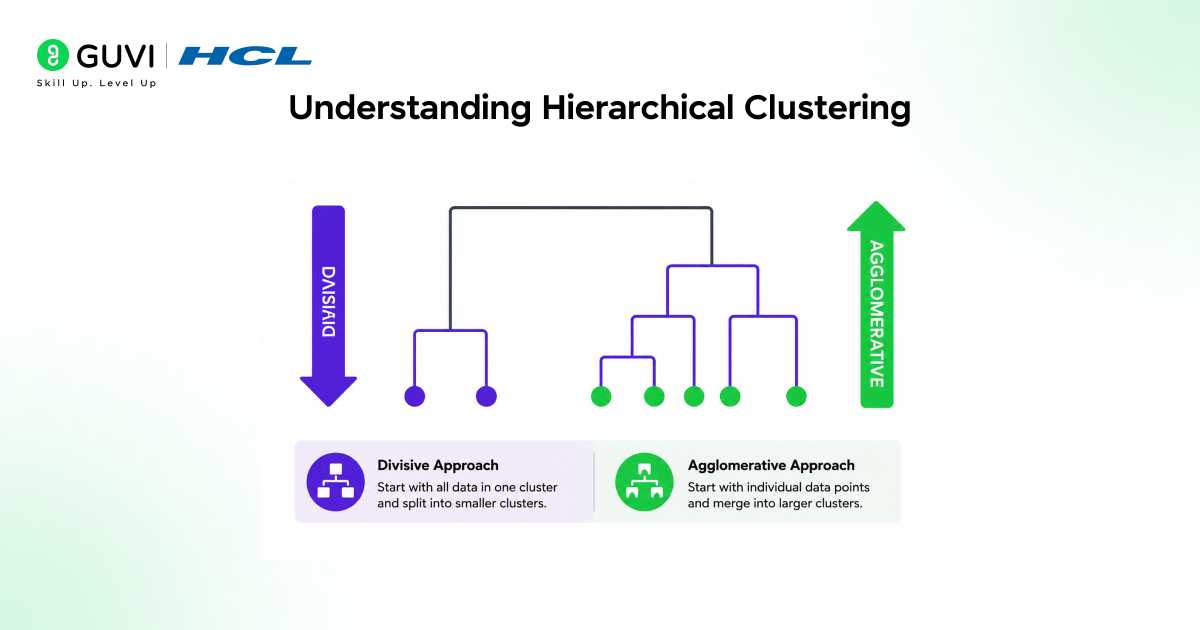
Hierarchical clustering builds a hierarchy of clusters. It mainly comes in two forms:
Agglomerative Hierarchical Clustering
This approach starts with individual points and merges them step by step.
Divisive Hierarchical Clustering
This approach starts with one large cluster and breaks it down into smaller clusters.
Among these two methods, agglomerative clustering is more popular because it is easier to use and more efficient.
How Bottom-Up Clustering Works
Bottom-up clustering involves these steps:
- Treat each data point as a separate cluster.
- Calculate the distance matrix for all clusters.
- Identify the two closest clusters.
- Merge those clusters.
- Update the distance matrix.
- Repeat until the desired number of clusters is formed.
The way the algorithm measures distances between clusters depends on the chosen linkage methods.
How Cluster Merging Happens in Agglomerative Clustering
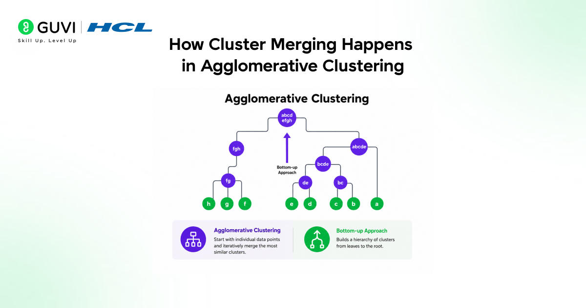
Cluster merging is the core process behind agglomerative clustering. Initially, every data point is its own cluster. The algorithm then calculates the distance between clusters and merges the two closest clusters.
After every merge, the distance matrix gets updated to reflect the newly formed cluster. This process continues repeatedly until the required number of clusters is achieved.
The merging behavior depends heavily on the selected linkage methods:
- Ward linkage focuses on minimizing cluster variance.
- Complete linkage uses the maximum distance between clusters.
- Single linkage uses the minimum distance between clusters.
- Average linkage considers the average distance between all points.
Because of this step-by-step merging structure, agglomerative clustering is considered a bottom-up clustering technique.
Types of Linkage Methods
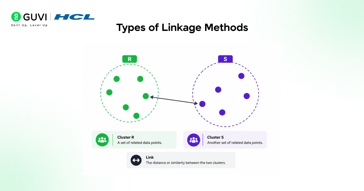
Linkage methods decide how the distance between two clusters is measured when they are merged.
1. Ward Linkage
Ward linkage merges the pair of clusters that causes the smallest increase in within-cluster variance, which tends to produce compact clusters of similar size. It is the default in sklearn’s AgglomerativeClustering and works only with Euclidean distance.
2. Complete Linkage
Complete linkage uses the largest distance between any two points, one from each cluster. This favors compact clusters, but a single distant point can inflate that maximum, so outliers still affect it.
3. Single Linkage
Single linkage uses the smallest distance between any two points across the clusters. It can follow elongated or irregular shapes, but noise and outliers can chain unrelated points into one cluster.
4. Average Linkage
Average linkage takes the mean distance across all point pairs between two clusters. It offers a middle ground between single and complete linkage.
In sklearn, you choose the method with the linkage parameter, using 'ward', 'complete', 'average', or 'single'.
Comparison of Linkage Methods in Agglomerative Clustering
| Feature | Ward | Complete | Single | Average |
|---|---|---|---|---|
| Distance Measured | Increase in within-cluster variance | Largest distance between points | Smallest distance between points | Mean of all pairwise distances |
| Cluster Shape | Compact, similar size | Compact, roughly round | Elongated, chain-like | Moderately compact |
| Outlier Sensitivity | High | High | Very high | Moderate |
| Metric Support | Euclidean only | Any supported metric | Any supported metric | Any supported metric |
| Best For | Evenly sized, compact clusters | Well-separated, compact clusters | Irregular shapes in clean data | A balanced choice when unsure |
Picking the right linkage and cut height gets easier with guided, hands-on work. HCL GUVI’s Intel & IITM Pravartak Certified AI/ML Course pairs live classes from industry experts with 20+ end-to-end projects, so ideas like clustering turn into skills you can confidently apply.
What is a Distance Matrix?
A distance matrix records the pairwise distances between all data points or clusters.
During agglomerative clustering, the algorithm updates the distance matrix after each merging step. The distance matrix plays a crucial role in deciding which clusters to merge next.
Common distance metrics include:
- Euclidean distance
- Manhattan distance
- Cosine distance
What is a Dendrogram?
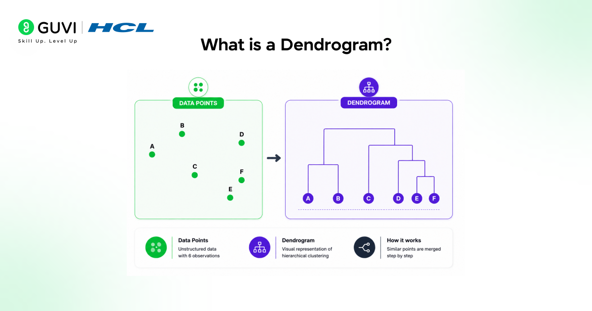
A dendrogram is a tree diagram that shows how hierarchical clustering merges data points, starting with each sample on its own and ending with one cluster.
- Leaves: Each leaf at the bottom represents a single data point.
- Merge Height: The height where two branches join shows the distance between those clusters, so taller joins mean less similar groups.
- Choosing Clusters: Cutting the tree with a horizontal line splits it into clusters, and a common rule of thumb is to cut across the longest vertical gap.
Sklearn does not draw this tree by itself, but SciPy’s dendrogram function makes it easy to plot.
Implementing Agglomerative Clustering using Sklearn
Now let us apply sklearn’s AgglomerativeClustering to a sample dataset.
Step 1: Import the Required Libraries
import matplotlib.pyplot as plt
from sklearn.datasets import make_blobs
from sklearn.cluster import AgglomerativeClusteringmatplotlib.pyplotdraws the plot.make_blobsgenerates a sample dataset.AgglomerativeClusteringis the clustering model.
Step 2: Create a Sample Dataset
X, y = make_blobs(
    n_samples=300,
    centers=4,
    cluster_std=1.2,
    random_state=42
)n_samples=300creates 300 data points.centers=4forms four groups.cluster_std=1.2controls how spread out each group is.random_state=42gives the same data on every run.
Step 3: Apply Agglomerative Clustering
model = AgglomerativeClustering(
    n_clusters=4,
    linkage='ward'
)
labels = model.fit_predict(X)n_clusters=4sets the number of clusters to find.linkage='ward'merges the pair of clusters that increases variance the least.fit_predictfits the model and returns a cluster label for each point.

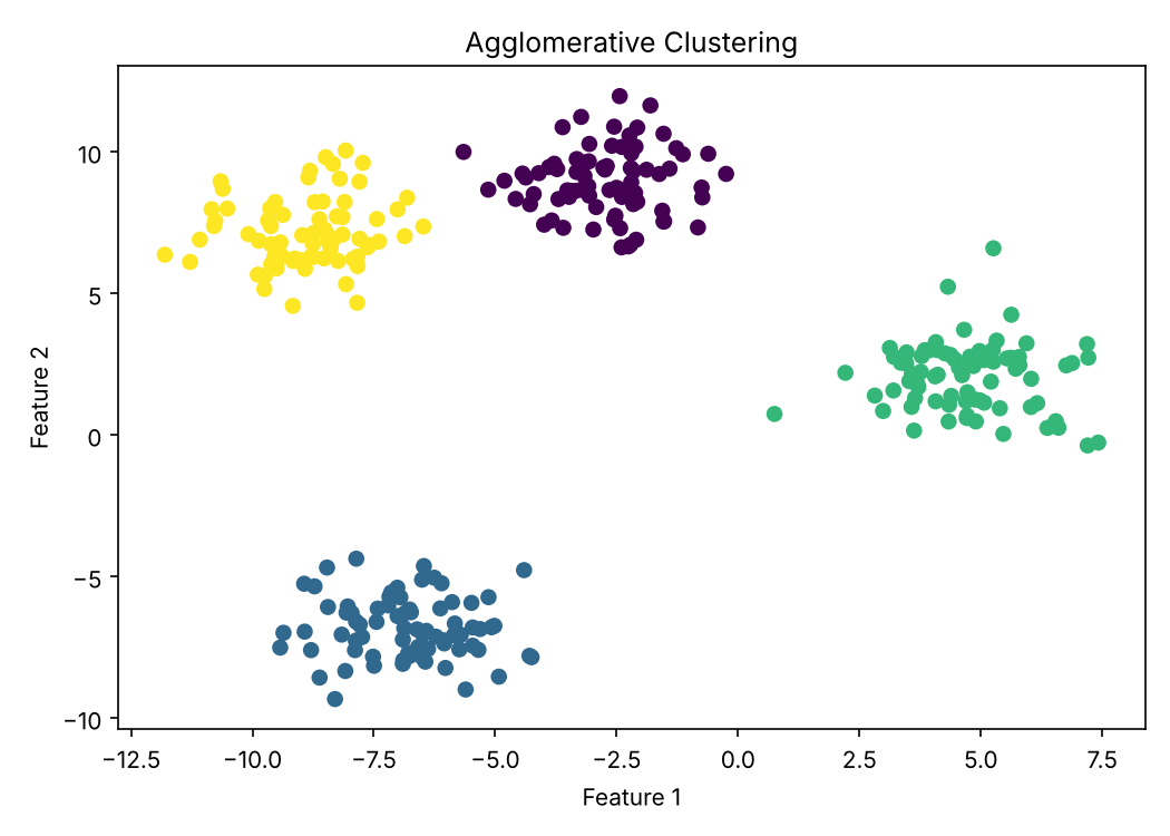
Step 4: Visualize the Clusters
plt.scatter(X[:, 0], X[:, 1], c=labels)
plt.title('Agglomerative Clustering')
plt.xlabel('Feature 1')
plt.ylabel('Feature 2')
plt.show()c=labelscolors each point by its cluster.- The title and axis labels make the plot easier to read.
Output:
Visualizing Clusters using a SciPy Dendrogram
A SciPy dendrogram shows how the data points merge into clusters, step by step. This section reuses X and plt from the previous section.
Step 1: Import SciPy Libraries
from scipy.cluster.hierarchy import dendrogram, linkagelinkagecalculates the merge steps.dendrogramdraws the tree from those steps.
Step 2: Create the Linkage Matrix
linked = linkage(X, method='ward')method='ward'matches the linkage used in the sklearn model.- The result has one row per merge, showing which two clusters joined and at what distance.
Step 3: Plot the Dendrogram
plt.figure(figsize=(10, 5))
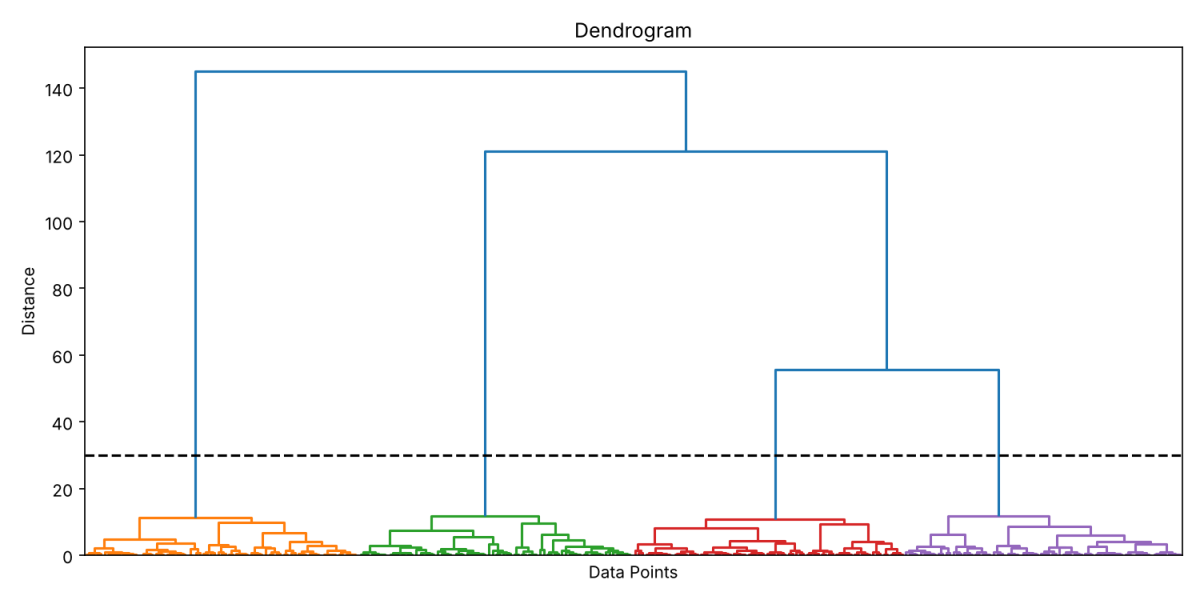
dendrogram(linked, no_labels=True, color_threshold=30)
plt.axhline(y=30, color='black', linestyle='--')
plt.title('Dendrogram')
plt.xlabel('Data Points')
plt.ylabel('Distance')
plt.show()no_labels=Truehides the 300 leaf labels, which would overlap.color_threshold=30gives each cluster below distance 30 its own color.plt.axhlinedraws a dashed cut line at distance 30.
Output:
How to Choose the Number of Clusters in Agglomerative Clustering
Unlike k-means, agglomerative clustering does not need the cluster count in advance. The full hierarchy is built first, and the count is decided afterwards using one of the methods below.
1. Cut the Dendrogram
Cut where the vertical gap between successive merges is largest. The number of branches the line crosses is the number of clusters.
from scipy.cluster.hierarchy import fcluster

labels = fcluster(linked, t=30, criterion='distance')
2. Set a Distance Threshold
Instead of a count, set the distance at which merging stops. The number of clusters then follows from the data.
model = AgglomerativeClustering(
    n_clusters=None,
    distance_threshold=30,
    linkage='ward'
)
labels = model.fit_predict(X)
3. Use the Silhouette Score
Fit the model for several cluster counts and score each one. The score ranges from -1 to 1, and the highest value marks the best-separated clusters.
from sklearn.metrics import silhouette_score

for k in range(2, 9):
    labels = AgglomerativeClustering(n_clusters=k).fit_predict(X)
print(k, silhouette_score(X, labels))| Method | Based On | Best For |
|---|---|---|
| Dendrogram cut | Largest merge gap | Visual, quick inspection |
| Distance threshold | A fixed merge distance | Unknown cluster count |
| Silhouette score | Cluster separation | Comparing candidate counts |
When the dendrogram and the silhouette score point to the same number, the choice is well supported.
Advantages of Agglomerative Clustering
Agglomerative clustering builds a hierarchy of clusters from the bottom up, which gives it several practical strengths.
- No Centroids Needed: It does not start from randomly placed centers, so results stay stable across runs.
- Flexible Cluster Count: Setting
distance_thresholdlets you skip choosing the number of clusters in advance. - Clear Dendrograms: The merge tree shows how clusters form at each distance, which makes the structure easy to read.
- Multiple Linkage Options: Ward, complete, average, and single linkage control how the distance between clusters is measured.
- Suits Smaller Datasets: It performs well on small to medium data, where computing all pairwise distances is affordable.
Limitations of Agglomerative Clustering
These drawbacks matter most when data is large, noisy, or constantly growing.
- High Computational Cost: Pairwise distances must be stored and updated, so memory and time rise quickly as the dataset grows.
- Sensitive to Outliers: Extreme points can distort merges, and single linkage may chain unrelated points into one cluster.
- Irreversible Merges: The algorithm is greedy, so an early merge cannot be corrected later.
- No Predict Method: Sklearn offers only
fitandfit_predict, so new samples cannot be assigned to existing clusters directly.
Real-World Applications of Agglomerative Clustering
Its hierarchical output suits problems where groups contain smaller sub-groups.
- Customer Segmentation: Separates buyers by habits such as purchase frequency and spend, and the dendrogram hints at how many segments exist.
- Document Clustering: Sorts articles, reviews, or support tickets by content similarity, often using cosine distance on text vectors.
- Image Segmentation: Merges neighboring pixels or regions of similar color or texture into coherent segments.
- Bioinformatics: Finds genes with similar expression patterns and shows how genes or species relate through dendrograms.
Understanding agglomerative clustering shows you can learn complex ideas, and that is exactly the mindset AI careers reward. HCL GUVI’s Intel & IITM Pravartak Certified AI/ML Course turns it into a career with live mentoring, 20+ projects, a capstone, and placement support. Take the step and start building!
Conclusion
Agglomerative clustering stands out because it exposes the nested structure of a dataset instead of a single flat partition. Its results are reproducible since no centroids are initialized, though storing pairwise distances limits its reach on large data. The linkage method and distance metric shape the clusters, so the outcome reflects the technique’s assumptions as much as the data.
FAQs
1. What is agglomerative clustering?
It is a bottom-up hierarchical method that starts with every point as its own cluster and repeatedly merges the closest pair until the stopping condition is met.
2. What is the difference between agglomerative and divisive clustering?
Agglomerative clustering builds clusters by merging from individual points upward, while divisive clustering begins with one cluster and splits it downward.
3. What is the difference between K-means and agglomerative clustering?
K-means needs a preset number of clusters and iteratively updates centroids, whereas agglomerative clustering needs no centroids and produces a full merge hierarchy.
4. How do you choose the number of clusters in agglomerative clustering?
Cut the dendrogram at the height where the vertical gap between successive merges is largest, or set a distance threshold.
5. What is the time complexity of agglomerative clustering?
The standard approach takes O(n³) time, or O(n² log n) with a priority queue, and requires O(n²) memory.
Success Stories
















Did you enjoy this article?