Pandas Introduction

Have you ever wondered how data professionals manage and analyze large datasets with ease? The answer lies in Pandas, one of the most powerful and popular Python libraries for data analysis and manipulation. Pandas makes it incredibly simple to clean, transform, and explore structured data all with just a few lines of code.

Whether you’re analyzing financial trends, preparing customer insights, or building machine learning models, Pandas provides the tools you need to handle data efficiently. Its user-friendly syntax and high performance have made it an essential part of every data science workflow.

In this blog, we’ll explore what Pandas in Python is, why it’s so widely used, and how it has revolutionized the way data is processed, analyzed, and visualized in today’s data-driven world.

What Is Pandas?

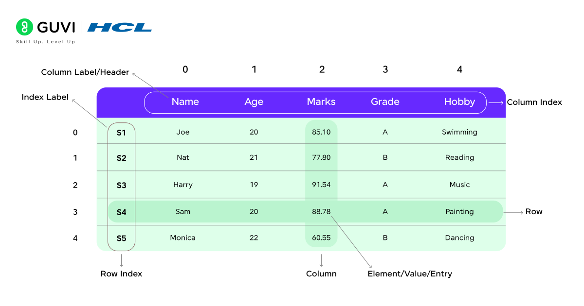
Pandas is an open-source Python library built specifically for data manipulation and analysis. The name Pandas comes from the term “Panel Data,” which refers to multi-dimensional structured datasets commonly used in statistics and economics.

It’s built on top of NumPy, which means it inherits NumPy’s speed and efficiency while adding powerful, user-friendly features for working with labeled tabular data. This makes it perfect for handling datasets from various sources such as CSV, Excel, SQL databases, or even JSON files.

Think of it this way — imagine you’re working with an Excel sheet containing thousands of rows and columns. Instead of manually scrolling, filtering, and sorting data, Pandas lets you perform these operations instantly using simple Python commands. With Pandas, managing large datasets becomes faster, cleaner, and far more efficient.

Why Use Pandas?

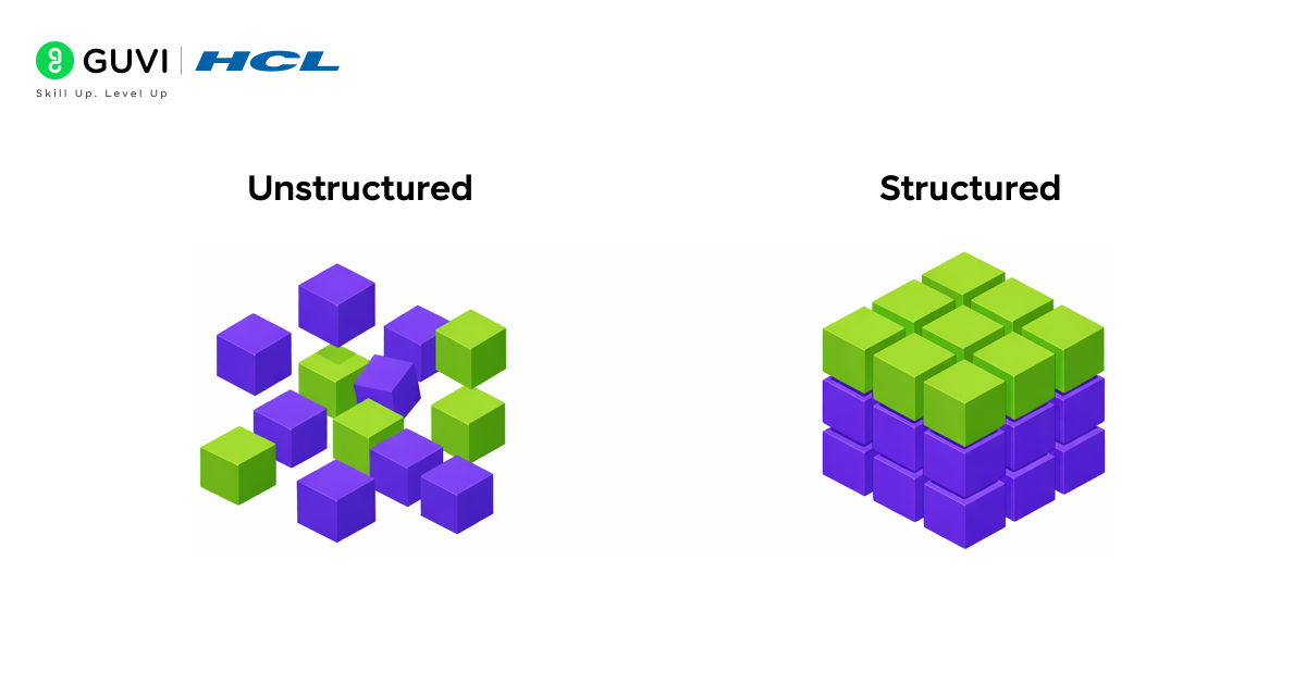
The real strength of Pandas lies in its speed, simplicity, and flexibility. It allows you to perform complex data manipulation tasks quickly and efficiently — things that would otherwise take hundreds of lines of code.

Here are some key reasons why Pandas is so widely used in data science:

• Efficient Data Handling: Pandas can process and manage large datasets smoothly without slowing down your system.
• Data Cleaning and Transformation: It helps remove duplicates, handle missing values, and reshape data easily for analysis.
• Quick Data Summaries: With a few commands, you can generate descriptive statistics and explore patterns in your data.
• Merging and Joining: Pandas allows you to combine multiple datasets from different sources seamlessly.
• Integration with Other Libraries: It works perfectly with libraries like Matplotlib, Seaborn, and Scikit-learn for visualization and machine learning.

For example, if you have a CSV file containing customer purchase data, you can read it, remove duplicates, calculate averages, and group data by region — all within a few lines of code. That’s why Pandas is considered a must-have tool for anyone working with data in Python.

Key Data Structures In Pandas

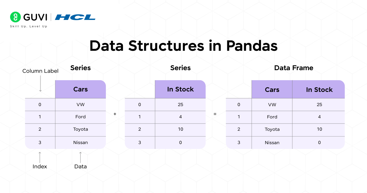
At the heart of Pandas are two key data structures — Series and DataFrame. These two form the foundation of all data handling and analysis tasks in Pandas. In this section, we’ll explore both in detail, understand how they work, their features, and see practical examples with code to help you get started easily.

1. Series

A Series in Pandas is a one-dimensional labeled array that can store data of any type — numbers, strings, or even objects. You can think of it as a single column of data in an Excel sheet or database table.

Each value in a Series is linked to an index label, making it simple to access, modify, or filter specific pieces of data. Series are commonly used for storing simple, structured data like prices, marks, or ratings.

Example:

import pandas as pd

data = pd.Series([10, 20, 30, 40], index=['A', 'B', 'C', 'D'])
print(data)

Output:
A    10
B    20
C    30
D    40
dtype: int64

Key Features of Pandas Series:

• Labeled Index: Each value has a label (index) for easy lookup and access.
• Homogeneous Data: Stores data of the same type, making operations faster and cleaner.
• Vectorized Operations: Perform mathematical or logical operations on all elements at once.
• Easy Indexing: Access elements by label or position effortlessly.

Example of Data Access:

# Access element using label
print(data['B'])

# Access element using position
print(data[2])

Why Use Series?

A Series in Pandas is perfect for handling one-dimensional data like prices, scores, or sales figures. It’s simple, fast, and comes with labeled indexes that make data access and filtering effortless.

You should use a Series when you want to:

• Work with a single column of data
• Perform quick calculations or summaries
• Access data easily using labels or positions

In short, Series are the easiest way to store and analyze one-dimensional data in Pandas.

2. DataFrame

A DataFrame is the most important and commonly used data structure in Pandas. It’s a two-dimensional table with rows and columns — much like an Excel sheet or SQL table. You can think of it as a collection of multiple Series objects that share the same row index.

Example:

import pandas as pd

data = {
    'Name': ['Alice', 'Bob', 'Charlie'],
    'Age': [25, 30, 35],
    'City': ['New York', 'London', 'Sydney']
}

df = pd.DataFrame(data)
print(df)
Output:
     Name  Age      City
0    Alice   25  New York
1      Bob   30    London
2  Charlie   35    Sydney

Key Features of Pandas DataFrame:

• Two-Dimensional Structure: Data is organized in rows and columns for better readability.
• Heterogeneous Data: Each column can contain different data types like numbers, text, or dates.
• Label-Based Indexing: Access rows and columns easily by their labels.
• Powerful Data Operations: Supports sorting, filtering, merging, grouping, and reshaping.
• Library Integration: Works seamlessly with visualization and machine learning tools.

Example Operations:

# Access a column
print(df['Name'])

# Add a new column
df['Salary'] = [50000, 60000, 70000]

# Filter rows where Age > 28
print(df[df['Age'] > 28])

Why to Use DataFrames?
A DataFrame is the core of data analysis with Pandas, designed for two-dimensional data like tables or spreadsheets. It helps you organize, clean, and analyze structured data efficiently.

Use a DataFrame when you need to:

• Manage datasets with multiple columns
• Merge, filter, or group data
• Prepare data for visualization or machine learning

Simply put, DataFrames make handling and analyzing real-world data in Python both easy and powerful.

Basic Operations In Pandas

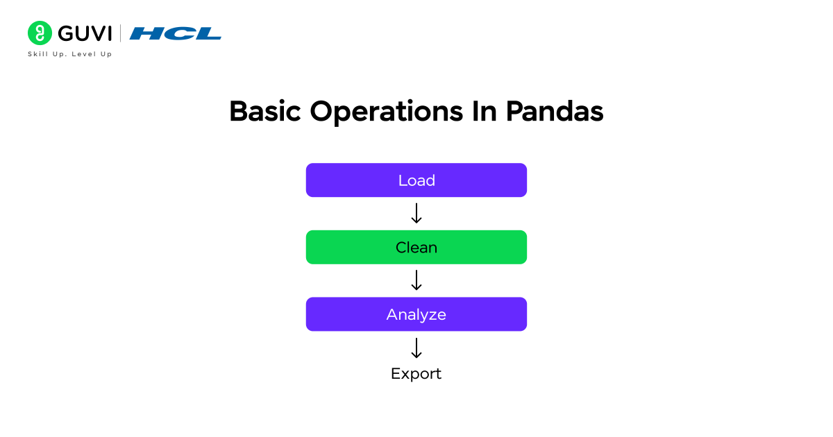
Now that you understand Pandas data structures, it’s time to explore how to work with them in real projects. In this section, we’ll look at some of the basic operations you’ll frequently use in data analysis with Pandas. These include:

• Reading and Writing Data – Loading data from different file formats and saving processed results.
• Viewing Data – Quickly checking the shape, summary, and structure of your dataset.
• Filtering Data – Selecting rows or columns based on specific conditions.
• Handling Missing Data – Detecting, removing, or filling gaps in your dataset.

These operations form the backbone of any data science workflow. Once you get comfortable with them, managing and analyzing large datasets becomes fast and intuitive. Let’s explore each operation in detail below.

1. Reading and Writing Data

Pandas makes it easy to import and export data across multiple formats such as CSV, Excel, and SQL databases. You can read raw data into a DataFrame and export cleaned results with just a few lines of code.

import pandas as pd
# Read a CSV file
df = pd.read_csv('data.csv')
# Read an Excel file
df_excel = pd.read_excel('data.xlsx')
# Write cleaned data back to a CSV
df.to_csv('output.csv', index=False)

2. Viewing Data

Before analyzing, it’s crucial to understand the structure of your data. Pandas provides quick functions to view sample rows, column information, and basic statistics.

df.head()       # Shows first 5 rows
df.tail()       # Shows last 5 rows
df.info()       # Displays column names and data types
df.describe()   # Gives summary statistics of numeric columns

3. Filtering Data

Filtering helps you focus only on the information you need. Whether you’re selecting rows with specific values or applying multiple conditions, Pandas makes it simple.

# Select rows where Age > 25
filtered = df[df['Age'] > 25]
# Filter with multiple conditions
filtered = df[(df['Age'] > 25) & (df['City'] == 'Delhi')]

4. Handling Missing Data

Real-world data often contains missing or incomplete values. Pandas offer straightforward ways to clean and fix them.

# Remove rows with missing values
df.dropna(inplace=True)
# Replace missing values with a default value
df.fillna(0, inplace=True)

For a more detailed and structured guide, download HCL GUVI’s Free Data Science eBook. It walks you through key topics such as Python programming, Pandas, NumPy, data visualization, and machine learning fundamentals. Each chapter includes clear explanations, examples, and tips to help you understand how data science is applied in real-world scenarios. It’s a perfect resource for self-paced learners who want to strengthen their foundation.

Data Cleaning And Manipulation

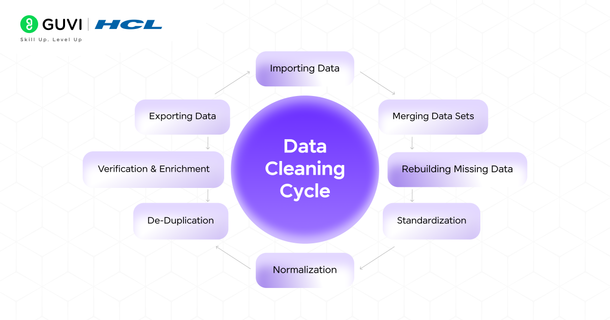
Real-world data is rarely perfect; it often comes with missing values, duplicate entries, or inconsistent formatting. That’s where Pandas come in. It provides quick and powerful tools to clean, organize, and prepare your data for deeper analysis or machine learning. In this section, we’ll explore the most common data cleaning and manipulation operations in Pandas, including:

• Renaming Columns – To make column names more readable and consistent.
• Removing Duplicates – To eliminate repeated or redundant data.
• Sorting Data – To arrange your dataset in a meaningful order.
• Grouping and Aggregation – To summarize and analyze data efficiently.

1. Renaming Columns

When your dataset has unclear or inconsistent column names, you can easily rename them for better readability.

df.rename(columns={'Name': 'Full Name'}, inplace=True)

This helps make your dataset more descriptive and easier to understand, especially when sharing or documenting your work.

2. Removing Duplicates

Duplicate entries can skew analysis and lead to incorrect results. Pandas provide a quick way to remove them.

df.drop_duplicates(inplace=True)

This ensures each row in your DataFrame is unique and accurate.

3. Sorting Data

Sorting helps you view and analyze your data in a meaningful order, such as from highest to lowest value.

df.sort_values(by='Age', ascending=False)

For instance, this command sorts the dataset by age, showing the oldest entries first.

4. Grouping and Aggregation

Grouping allows you to summarize and analyze data based on specific categories — perfect for generating insights.

df.groupby('Department')['Salary'].mean()

For example, if you have employee data, this command groups employees by department and calculates the average salary for each group in seconds.

Data Selection And Indexing

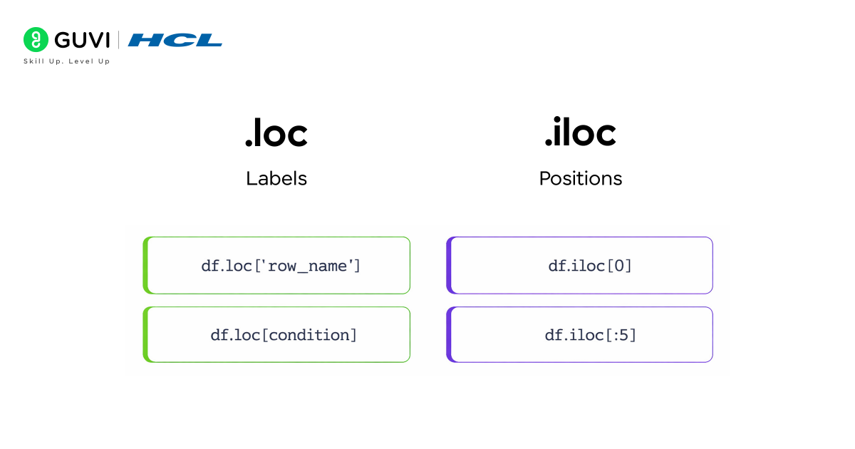
Selecting the right portion of data is one of the most powerful features of Pandas. Whether you want to extract a few columns, specific rows, or filter records based on conditions, Pandas gives you flexible and efficient ways to access exactly what you need. In this section, we’ll explore key data selection and indexing operations in Pandas, including:

• Selecting Columns
• Selecting Rows by Index
• Conditional Selection

Let’s break each of them down in detail.

1. Selecting Columns

In Pandas, columns represent attributes or features of your dataset — like Name, Age, or Salary. You can access them directly by using their names. 

1. If you want to view a single column, you can simply call it using square brackets:

# Select a single column
df['Name']

This returns a Series, which behaves like a single column of data.

2. To view multiple columns together, pass a list of column names inside double brackets:

# Select multiple columns
df[['Name', 'Age', 'Department']]

This returns a DataFrame with only the specified columns.

Example:
If you’re analyzing an employee dataset, you might only need the Name and Department columns to check team distribution. Pandas make this quick and clean.

2. Selecting Rows by Index

Rows represent individual records or entries in your dataset. Pandas provides two powerful indexing methods to select them: loc and iloc.

Using loc (Label-Based Selection) 

• loc allows you to access rows and columns using their labels (names).
• Ideal when your DataFrame has custom indexes or named rows.

# Select row using label
df.loc[0]

 You can also select a specific cell or range:

 df.loc[0, 'Name']       # Single cell
df.loc[0:3, ['Name', 'Age']]  # Range of rows and columns

Using iloc (Integer-Based Selection)

• iloc works with integer positions (like list indices).
• Perfect when you want to access rows or columns by number.

# Select row using integer index
df.iloc[0]
df.iloc[0:3, 1:3]

Example:
If you want to check the first five records in a large dataset or extract specific rows by number, iloc is the simplest approach.

Conditional Selection

One of the most powerful features of Pandas is the ability to filter rows based on conditions — just like SQL queries. This helps you analyze specific subsets of your data easily.

# Select rows where Age > 25
df[df['Age'] > 25]
# Multiple conditions
df[(df['Age'] > 25) & (df['Department'] == 'IT')]

Here’s what’s happening:

• The condition inside the brackets (df[‘Age’] > 25) returns a Boolean Series — True for rows that meet the condition.
• Pandas uses this to select only the matching rows.

Example:
Suppose you have an employee dataset. You can quickly filter employees above age 25 who belong to the IT department. This capability allows for dynamic and highly efficient data exploration without writing complex loops or conditional statements.

Merging, Joining, And Concatenation

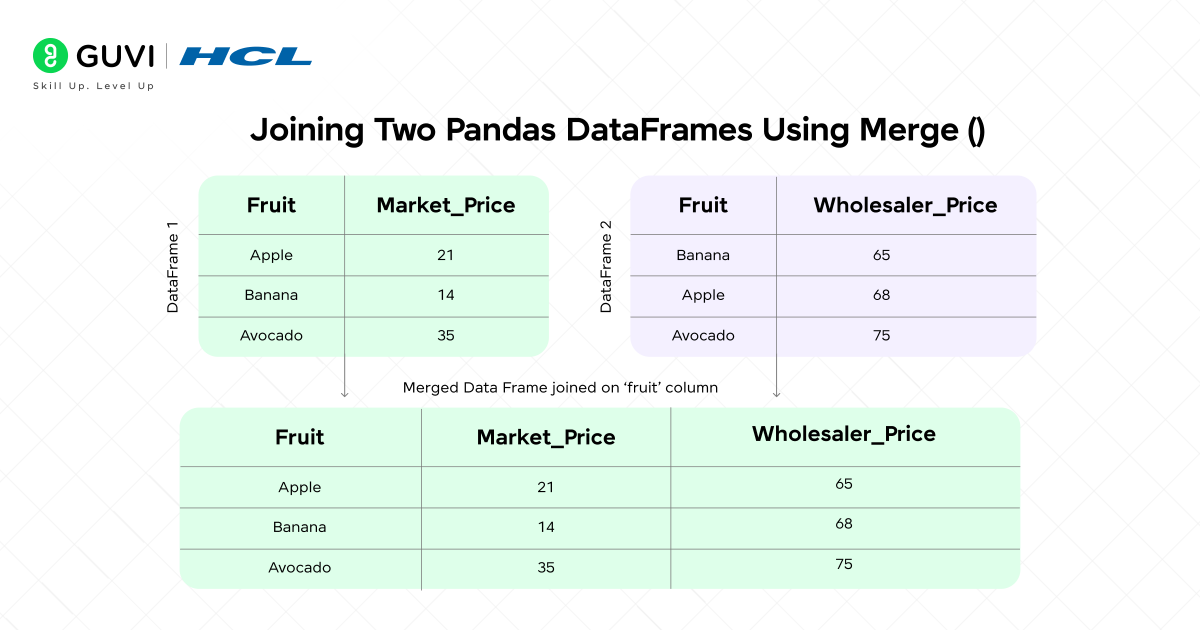
In real-world data projects, you rarely work with a single clean dataset. Data often comes from multiple sources — such as different Excel files, databases, or APIs. Pandas makes it incredibly easy to bring all these pieces together using merging, joining, and concatenation. These operations allow you to combine datasets efficiently for deeper and more meaningful analysis.

In this section, we’ll explore three key methods:

• Concatenation – Stacking multiple DataFrames together.
• Merging – Combining DataFrames based on a common column.
• Joining – Linking DataFrames using their indexes.

1. Concatenation

Concatenation is used to stack DataFrames either vertically (one below another) or horizontally (side by side). It’s perfect when you have data split across multiple files or time periods that need to be combined.

import pandas as pd
combined = pd.concat([df1, df2])

You can also use axis=1 to join columns side by side:

combined = pd.concat([df1, df2], axis=1)

Example:
If you have sales data for January and February in two separate DataFrames, you can concatenate them to create a full quarterly report in seconds.

2. Merging

Merging is similar to SQL joins — it lets you combine DataFrames based on a common column or key. It’s one of the most commonly used methods in data integration tasks.

merged = pd.merge(df1, df2, on='EmployeeID')

You can also specify the type of merge (inner, outer, left, right) depending on how you want to handle unmatched rows.

merged = pd.merge(df1, df2, on='EmployeeID', how='outer')

Example:
You might merge an employee details DataFrame with another containing performance reports using the EmployeeID column as the common key — all in a single line of code.

3. Joining

Joining is a more convenient way to combine DataFrames using their index values instead of columns. It’s especially useful when working with time series or indexed data.

joined = df1.join(df2)

You can also control the type of join (like in SQL):

joined = df1.join(df2, how='inner')

Example:
If one DataFrame contains employee names indexed by ID and another contains department data with the same index, a join quickly brings them together.

Real-World Applications Of Pandas

Pandas powers countless real-world data applications. Here are a few domains where it shines:

• Finance: Analyze stock data, calculate moving averages, and assess trends.
• Healthcare: Manage patient records and predict disease patterns.
• Marketing: Track campaign performance and customer engagement.
• Education: Monitor student performance metrics.
• E-Commerce: Analyze purchase patterns to improve recommendations.

If you enjoy learning step by step, HCL GUVI’s 5-Day Free Data Science Email Series is a great way to begin your data journey. Each day, you’ll receive short, practical lessons that cover Python basics, Pandas operations, and real-world examples you can try yourself. It’s designed to help beginners build a solid understanding of data science concepts through simple, hands-on exercises.

Advantages And Limitations Of Pandas

Like any tool, Pandas has its own advantages and limitations. Understanding both helps you use it effectively and know when to pair it with other tools.

Advantages of Pandas

• Easy to Learn and Use: Pandas has a simple, human-readable syntax that makes data manipulation quick, even for beginners.
• Efficient for Structured Data: It’s perfect for working with structured data like CSVs, Excel sheets, or SQL tables.
• Powerful Data Cleaning and Transformation: Pandas provides built-in functions to handle missing values, remove duplicates, and reshape data effortlessly.
• Seamless Integration: It works smoothly with other Python libraries such as NumPy, Matplotlib, and Seaborn, making it a complete data analysis toolkit.

Limitations of Pandas

• Not Ideal for Very Large or Real-Time Data: Pandas is designed for in-memory processing, so handling massive or streaming datasets can be slow.
• High Memory Consumption: Large DataFrames may use significant RAM, which can cause performance issues on low-end systems.
• Complexity for Advanced Tasks: While basic operations are easy, mastering multi-level indexing, merges, or performance tuning can take time.

Conclusion

Pandas is one of the most essential tools in data science and data analysis. It allows you to clean, organize, and explore data easily using simple Python commands. Whether you’re fixing missing values, sorting records, or combining datasets, Pandas helps you handle everything quickly and efficiently. It works perfectly with data from different sources like CSV files, Excel sheets, and databases, making it a reliable choice for almost any data-related task.

Beyond just simplifying data handling, Pandas gives you the power to perform detailed analysis and uncover insights without writing long or complicated code. It’s useful for beginners who are learning data analysis as well as professionals managing large datasets. By mastering Pandas, you build a strong foundation for working confidently with real-world data and take an important step toward becoming skilled in data science.

Do consider enrolling in HCL GUVI’s Data Science Course to learn data science in depth. This mentor-led program offers a structured learning path, real-world projects, hands-on Python and Pandas training, interview preparation, and placement assistance — helping you transition from learner to job-ready professional.

FAQs

1. Can Pandas Handle Real-Time Data?

Pandas is great for batch data processing but not designed for real-time streaming. For real-time pipelines, libraries like PySpark or Dask are preferred.

2. Is Pandas Enough For Data Science Jobs?

 It’s a foundational skill. Pairing Pandas with SQL, visualization, and machine learning tools will make you job-ready.

3. What’s The Difference Between Pandas And NumPy?

NumPy handles numerical computations, while Pandas builds on it to manage labeled, structured data like tables and CSV files.

4. Can Pandas Be Used With Visualization Tools?

Yes. It integrates seamlessly with Matplotlib, Seaborn, and Plotly for building charts and plots.

5. Is Pandas Suitable For Beginners?

Absolutely. Pandas is one of the most beginner-friendly libraries, making it ideal for anyone entering the data analysis field.