
A Complete Guide to Regularization in Machine Learning: L1, L2, and Beyond for Reducing Overfitting
Oct 04, 2025 8 Min Read 3075 Views
(Last Updated)
Ever wondered why a machine learning model performs flawlessly on training data but crumbles the moment it faces new information? That silent killer is overfitting and the antidote is regularization. Regularization in machine learning is the difference between a flashy model that fails in the real world and a reliable one that consistently delivers.
In this guide, we’ll break down the role of regularization in ML. We will explore the bias-variance tradeoff and show practical regularization examples in both classic models and deep learning. If you’ve ever asked, “What is regularization in machine learning, and why does it matter?”, then you’re in the right place. Keep reading to find out how regularization can remake your ML models from fragile experiments into robust solutions.
Table of contents
- What is Regularization in Machine Learning?
- Types of Regularization in Machine Learning
- L1 Regularization (Lasso Regression)
- L2 Regularization (Ridge Regression)
- Elastic Net Regularization
- Regularization in Deep Learning Models
- Top Tools for Applying Regularization in Machine Learning
- What are Overfitting, Appropriate Fitting, and Underfitting?
- Comparison of Overfitting, Appropriate Fitting, and Underfitting
- What are Bias and Variance in Machine Learning?
- Top Benefits of Regularization in Machine Learning
- How Regularization Shapes Real-World Machine Learning Models?
- Conclusion
- FAQs
- Why is regularization important in machine learning?
- Which is better: L1 or L2 regularization?
- Can regularization cause underfitting?
- How is regularization applied in neural networks?
- Is regularization in ML always needed?
What is Regularization in Machine Learning?
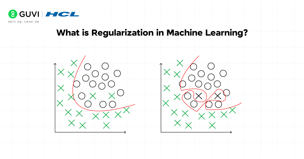
Regularization in machine learning is a set of mathematical techniques that control the complexity of a model to reduce overfitting. It works by adding a penalty term to the loss function so that the model does not assign excessively high weights to certain features. A model that fits training data too closely tends to capture noise instead of meaningful patterns, which weakens its ability to generalize. Regularization addresses this by shrinking coefficients in linear models or constraining weights in neural networks.
Regularization in deep learning often takes the form of dropout or weight decay. It prevents large parameter values from dominating the learning process. The role of regularization in ML extends beyond mathematics because it directly influences the bias-variance tradeoff and determines whether a model performs reliably on unseen data.
Read: Machine Learning Vs Deep Learning: A Layman’s Guide to AI in Easy Words
Types of Regularization in Machine Learning
Regularization methods shape the behavior of models by constraining parameter growth. They control how weights adapt to data and protect against overfitting.
Each type applies a distinct mathematical penalty, which changes both the training process and the interpretation of the final model. Here are the main approaches.
1. L1 Regularization (Lasso Regression)
L1 regularization works by adding the absolute values of coefficients to the cost function. This makes the optimization surface sharp, which forces weaker coefficients toward zero. As a result, many predictors are removed entirely. The model that remains is sparse and interpretable. Lasso regression is the most recognized form of L1 regularization and is used when feature selection is as important as prediction accuracy.
- Cost Function
J(β) = (1/2n) Σ (yᵢ – ŷᵢ)² + λ Σ |βⱼ|
Where
- Prediction error measured by mean squared error
- λ: penalty parameter that decides how strongly coefficients are penalized
- Σ |βⱼ|: absolute values of coefficients forming the L1 penalty
Top Features of L1 Regularization
- Produces sparse models with only essential predictors
- Performs built-in feature selection
- Reduces noise from irrelevant inputs
Best Use Cases of L1 Regularization (Lasso Regression)
- High-dimensional datasets where many predictors are irrelevant
- Problems where interpretability and feature selection are important
- Situations where sparse solutions reduce computation and simplify the model
Pros of L1 Regularization
- Creates models that are easier to interpret
- Removes predictors that do not contribute useful information
Cons of L1 Regularization
- Performs poorly with correlated variables
- May discard predictors that add value only when grouped together
2. L2 Regularization (Ridge Regression)
L2 regularization modifies the cost function by adding the square of coefficients. The penalty increases quadratically as coefficients grow. Large coefficients are reduced, while smaller ones shrink less aggressively. Ridge regression applies this method to stabilize models and reduce variance. It is most effective when predictors are correlated and all variables contribute to the outcome in some degree.
- Cost Function
J(β) = (1/2n) Σ (yᵢ – ŷᵢ)² + λ Σ βⱼ²
Where
- Prediction error measured by mean squared error
- λ: tuning parameter that adjusts penalty strength
- Σ βⱼ²: squared coefficients representing the L2 penalty
Top Features of L2 Regularization
- Retains all predictors even after shrinkage
- Provides stable coefficients under multicollinearity
- Produces smoother optimization compared to L1
Best Use Cases of L2 Regularization
- Regression tasks with multicollinearity among predictors
- Scenarios where all predictors carry some contribution to the output
- Cases where prediction accuracy is more important than model simplicity
Pros of L2 Regularization
- Improves generalization by reducing variance
- Stabilizes regression estimates in correlated data
Cons of L2 Regularization
- Retains irrelevant variables in the final model
- Does not remove predictors, which reduces interpretability
Read: Top 10 Types of Regression in Machine Learning You Must Know
3. Elastic Net Regularization
Elastic net combines the penalties of L1 and L2. It benefits from sparsity of lasso and stability of ridge. Models trained with an elastic net can keep groups of correlated predictors instead of discarding them. This balance makes it particularly effective in datasets where many predictors are present and some are interdependent.
- Cost Function
J(β) = (1/2n) Σ (yᵢ – ŷᵢ)² + λ₁ Σ |βⱼ| + λ₂ Σ βⱼ²
Where
- Mean squared error that measures prediction error
- λ₁: penalty parameter for the L1 part controlling sparsity
- λ₂: penalty parameter for the L2 part controlling stability
Top Features of Elastic Net
- Balances between feature selection and stability
- Retains correlated predictors in groups
- Flexible penalty structure with tunable parameters
Best Use Cases of Elastic Net Regularization
- Datasets with many correlated predictors that should be kept together
- Applications requiring both feature selection and coefficient stability
- Large-scale problems in bioinformatics, text, or finance where variables interact in groups
Pros of Elastic Net
- Handles datasets with correlated features better than lasso
- Produces balanced models suited for complex data
Cons of Elastic Net
- Requires careful tuning of both λ parameters
- Increases computational complexity with large datasets
Regularization in Deep Learning Models
Classical techniques such as L1, L2, and elastic net control complexity in linear and tree-based models. Deep learning requires its own methods because neural networks contain millions of parameters. Here are two of the most widely used approaches in deep learning regularization.
- Dropout
Dropout is a regularization method that reduces overfitting in neural networks. It works by deactivating a random fraction of neurons during training. This prevents the network from depending too heavily on specific neurons and forces learning to be distributed across many connections.
A probability value determines which neurons remain active in each training step. At test time, all neurons are restored, but their outputs are scaled to match the average effect during training. This makes predictions stable and reliable across unseen data.
Benefits
- Reduces overfitting in deep architectures
- Improves model robustness across new inputs
Limitations
- Training may take longer to converge
- High dropout rates can reduce accuracy
Read: Object Detection using Deep Learning: A Practical Guide
- Weight Decay
Weight decay applies an L2 penalty to network weights during training. It discourages large parameters by shrinking them slightly in each optimization step. This prevents a single weight from dominating predictions and keeps the model balanced.
The penalty term is added to the loss function, which modifies the gradient update rule. This steady shrinkage of parameters creates smoother optimization and helps the network generalize better to unseen data.
Benefits
- Improves stability of learning in large networks
- Keeps weight values within practical limits
Limitations
- Excessive penalty strength can lead to underfitting
- Requires careful tuning for each dataset and architecture
Master the art of building robust machine learning models with Artificial Intelligence and Machine Learning Course, powered by Intel Certification. Just like regularization keeps models from overfitting, this course equips you with the right balance of AI concepts, hands-on ML projects, deep learning applications, and MLOps practices to ensure your skills generalize well in real-world scenarios. With industry mentors, placement support, and globally recognized certification, this program transforms your passion for AI into a career-ready toolkit that helps you solve real business problems with confidence. Take the leap into mastering AI & ML with HCL GUVI today!
Top Tools for Applying Regularization in Machine Learning
Regularization techniques are supported by a wide range of tools and frameworks. These platforms simplify implementation and allow practitioners to apply methods such as L1, L2, dropout, and elastic net across different algorithms. Here are the most widely used tools.
- Scikit-learn
Scikit-learn is one of the most popular machine learning libraries in Python. It provides built-in support for ridge, lasso, and elastic net regularization within its linear models. Logistic regression and support vector machines in scikit-learn also include regularization parameters that can be tuned directly.
Highlights
- Simple API for ridge, lasso, and elastic net
- Consistent interface for hyperparameter tuning with GridSearchCV
- Works well for regression and classification tasks
- TensorFlow
TensorFlow supports advanced regularization techniques for deep learning. Weight decay and dropout can be applied within Keras layers using parameters such as kernel_regularizer or Dropout. TensorFlow also integrates seamlessly with optimizers that control weight penalties during training.
Highlights
- Flexible implementation of L1 and L2 regularization
- Dropout layers integrated into neural networks
- Scales well for production-level deep learning models
- PyTorch
PyTorch offers modular support for regularization. L1 and L2 penalties can be added through loss functions or optimizers. Dropout is available as a built-in layer and can be applied in both feedforward and convolutional architectures. Its dynamic computation graph makes experimentation straightforward.
Highlights
- Built-in dropout and weight decay support
- Optimizer parameters allow direct control of penalties
- Widely adopted in research and production
- XGBoost
XGBoost is a gradient boosting framework that incorporates regularization as part of its core design. Both L1 and L2 penalties are supported through parameters such as alpha and lambda. This reduces overfitting in boosted tree ensembles and makes models more generalizable.
Highlights
- Built-in L1 and L2 penalties for controlling tree complexity
- Highly effective for tabular datasets
- Regularization parameters allow fine-grained tuning
- LightGBM
LightGBM is another gradient boosting framework optimized for speed and memory efficiency. It provides regularization through parameters like lambda_l1, lambda_l2, and min_data_in_leaf. These help prevent overfitting in large-scale boosting tasks.
Highlights
- Fast training with large datasets
- Regularization built into boosting structure
- Strong performance in competitions and applied systems
What are Overfitting, Appropriate Fitting, and Underfitting?
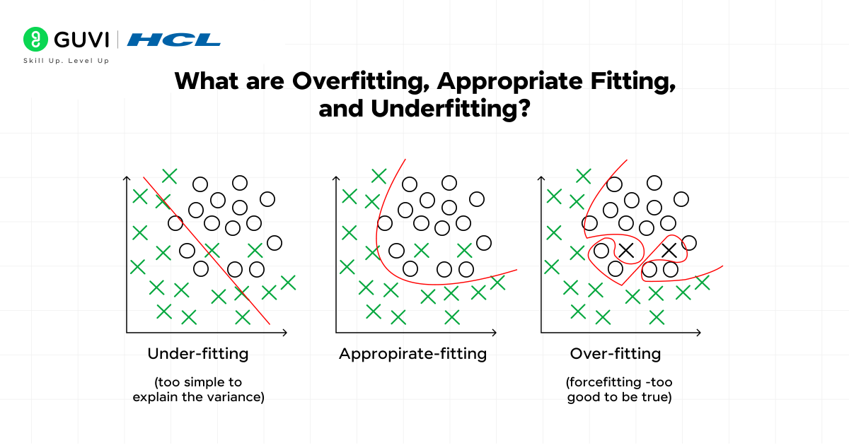
- Overfitting in Machine Learning
Overfitting happens when a model learns training data too closely. It memorizes patterns that are specific to the dataset, including noise and random fluctuations. The result is a model that performs well on training data but fails to generalize to new inputs.
Key Characteristics
- Very low training error but high test error
- Model is too complex for the amount of data
- Predictions are unstable when data changes
Where It Appears Most
- Small datasets with high model complexity
- Models trained for too many iterations
- Scenarios where regularization is weak or absent
- Appropriate Fitting in Machine Learning
Appropriate fitting describes the balanced state of a model. It captures meaningful patterns from the data without memorizing noise. The model performs consistently on both training and unseen datasets.
Key Characteristics
- Training error and test error remain close
- Model complexity matches dataset size and variability
- Predictions remain stable with new data
Where It Appears Most
- Well-regularized models tuned with proper hyperparameters
- Datasets with enough samples to reflect the true distribution
- Scenarios where model capacity is aligned with problem difficulty
- Underfitting in Machine Learning
Underfitting occurs when a model is too simple to represent the underlying patterns in data. It fails to capture relationships and delivers poor performance on both training and test datasets.
Key Characteristics
- High training error and high test error
- Model lacks flexibility or expressive power
- Predictions ignore meaningful trends
Where It Appears Most
- Models trained with very few features
- Algorithms with insufficient complexity for the task
- Scenarios where data preprocessing is weak or incomplete
Comparison of Overfitting, Appropriate Fitting, and Underfitting
| Feature | Overfitting | Appropriate Fitting |
| Error Pattern | Very low training error but high test error | Training error and test error remain close |
| Model Complexity | Too complex relative to the data | Balanced with dataset size and variability |
| Main Cause | Model learns noise and spurious details | Model captures true structure of data |
| Outcome | Strong on training set but weak on unseen data | Performs well on both training and test data |
| Practical Signs | Predictions change drastically with new inputs | Predictions remain stable across datasets |
| Best Remedy | Apply regularization, gather more data, or simplify the model | Maintain current setup with careful monitoring |
What are Bias and Variance in Machine Learning?
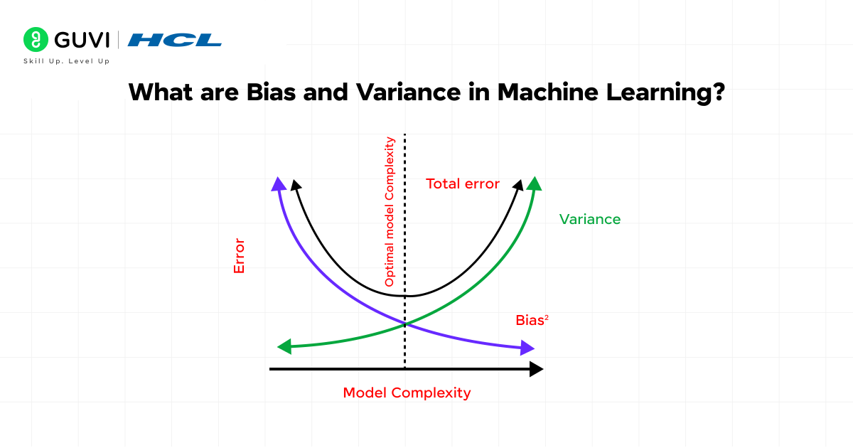
Bias and variance in machine learning describe two fundamental sources of error in machine learning models. They explain why models fail to generalize and highlight the tradeoff that guides model selection. A balanced model manages both bias and variance effectively.
- Bias in Machine Learning
Bias is the error introduced by making strong assumptions about the data. A model with high bias is too rigid and fails to capture important relationships. It oversimplifies the problem and produces systematic errors.
Key Characteristics of High Bias
- Predictions are consistently far from actual outcomes
- Training error remains high
- Model ignores complexity in the data
Where It Appears Most
- Very simple models such as linear regression applied to nonlinear problems
- Underfitting scenarios where the model lacks flexibility
- Cases where critical features are missing or ignored
- Variance in Machine Learning
Variance is the error introduced by sensitivity to training data. A model with high variance reacts strongly to small fluctuations in the dataset. It captures noise as if it were part of the pattern.
Key Characteristics of High Variance
- Very low training error but high test error
- Predictions change drastically when new data is introduced
- Model fits noise along with the signal
Where It Appears Most
- Very complex models such as deep trees without pruning
- Overfitting scenarios where the model memorizes the training data
- Cases where regularization is absent or too weak
Top Benefits of Regularization in Machine Learning
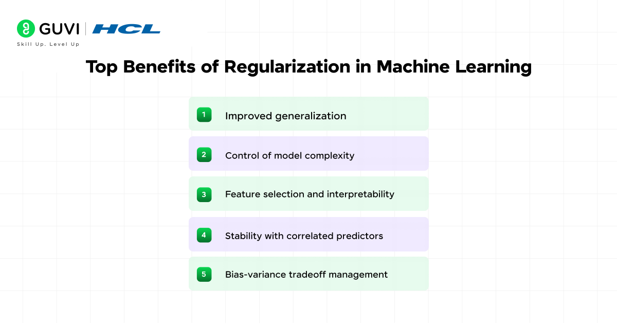
Here are the most important benefits that regularization provides to machine learning models. Each benefit explains why regularization is essential in both classical algorithms and deep learning models.
- Improved Generalization
Regularization improves the ability of models to generalize beyond training data. A model that fits training samples too closely often captures noise instead of meaningful patterns. Adding regularization penalizes overly large weights, which forces the model to rely on stronger and more stable relationships. This results in better performance when the model encounters unseen data, which is the true measure of its effectiveness.
- Control of Model Complexity
Regularization prevents models from becoming unnecessarily complex. Large coefficients make models highly sensitive to minor fluctuations in data. Regularization aligns the complexity of the model with the size and richness of the dataset by constraining weight growth. This balance reduces instability and produces models that learn essential structures instead of irrelevant details.
- Feature Selection and Interpretability
Regularization supports simpler and more interpretable models. L1 regularization in particular can eliminate irrelevant features by driving their coefficients to zero. The result is a model that focuses on fewer but more meaningful predictors. Such models are easier to interpret, which is valuable in applied fields like healthcare or finance where clarity is as important as accuracy.
- Stability with Correlated Predictors
Regularization improves stability in datasets where predictors overlap in information. Highly correlated features can cause coefficient estimates to fluctuate widely. Methods such as ridge regression and elastic net distribute influence across predictors and reduce this instability. A more stable model leads to predictions that remain consistent even when the input data shifts slightly.
- Bias-Variance Tradeoff Management
Regularization provides a direct way to manage the bias-variance tradeoff. Without it, models can swing toward overfitting or underfitting depending on complexity. Adding a regularization term increases bias slightly but reduces variance sharply. This shift creates models that are more balanced and captures important trends without being misled by noise.
How Regularization Shapes Real-World Machine Learning Models?
Regularization is not limited to theory. Its importance becomes clear in real-world systems where data is messy and decisions carry consequences. Below are practical domains where regularization strengthens machine learning models.
- Regularization in Recommendation Systems
Recommendation systems rely on data collected from millions of user interactions. These records often contain rare events that do not reflect long-term behavior. Without regularization, the model assigns extreme importance to these anomalies and produces unstable suggestions. Regularization reduces this problem by shrinking coefficients and focusing attention on consistent patterns.
Applications
- Keeps recommendations aligned with general user behavior
- Reduces over-reliance on outlier activity
- Supports long-term stability of ranking engines
- Regularization in Healthcare Models
Healthcare datasets combine diagnostic records and lab results. They also include missing entries and redundant variables. A model without regularization treats all features equally, which hides the most critical clinical indicators. L1 regularization addresses this by removing predictors with weak influence and emphasizing stronger ones.
Applications
- Highlights meaningful biomarkers that support clinical analysis
- Produces simpler models that doctors can interpret
- Improves trust in machine learning predictions used in care settings
- Regularization in Finance
Financial models must process variables such as stock prices and credit indicators. These predictors are often correlated, which makes raw regression unstable. Elastic net provides a balanced approach that keeps related predictors together while shrinking irrelevant ones. This improves predictive stability and reduces the chance of sudden swings in model output.
Applications
- Provides consistent risk assessment under market fluctuations
- Retains meaningful clusters of financial features
- Reduces noise created by short-lived signals
- Regularization in Deep Learning Applications
Neural networks contain millions of parameters. This size increases the risk of memorizing training data instead of learning useful features. Dropout improves learning by deactivating some neurons during training, which spreads influence across the network. Weight decay penalizes large weights and controls parameter growth. Data augmentation expands the dataset through variations such as rotations or shifts, which improves generalization.
Applications
- Prevents overfitting in large networks
- Builds robustness for vision and speech recognition tasks
- Produces reliable performance across different input conditions
Also Read: The Machine Learning Cheat Sheet [2025 Guide]
Conclusion
Regularization in ML is the foundation of building models that last beyond the training stage. A model that performs well in practice must balance complexity, control variance, and focus on meaningful features. Regularization provides that balance.
From classical approaches like lasso, ridge, and elastic net to deep learning methods such as weight decay and dropout, each technique addresses a specific weakness in model training. Their role extends from reducing noise in healthcare predictions to stabilizing financial risk models and powering large-scale recommendation engines.
The central idea is consistent. Without regularization, models collapse when faced with new data. With regularization, they become reliable tools that adapt to change and deliver results.
FAQs
Why is regularization important in machine learning?
It reduces overfitting and helps models generalize better to unseen data.
Which is better: L1 or L2 regularization?
L1 is preferred for feature selection, while L2 is suited for stability with correlated predictors.
Can regularization cause underfitting?
Yes. If the penalty is too strong, the model may oversimplify and fail to capture patterns.
How is regularization applied in neural networks?
It is often applied through weight decay or techniques such as dropout.
Is regularization in ML always needed?
No. Models trained on large datasets with low complexity may perform well without it, but most real-world tasks benefit from regularization.


Did you enjoy this article?