
Feature Selection Techniques in Machine Learning
Oct 28, 2025 7 Min Read 12432 Views
(Last Updated)
Feature selection techniques in machine learning profoundly impact model performance and efficiency. You’ve likely encountered the challenge of dealing with large datasets containing numerous features, where not all variables contribute equally to predicting the target variable.
This is where feature selection comes into play, helping you identify the most relevant attributes to build a robust machine-learning model. In this article, you’ll explore various feature selection techniques in machine learning, covering both supervised and unsupervised learning approaches.
Table of contents
- Understanding Feature Selection in Machine Learning
- Importance of Feature Selection
- Types of Feature Selection Techniques
- Supervised Feature Selection Methods
- 1) Filter-based Methods
- 2) Wrapper-based Methods
- 3) Embedded Approach
- Unsupervised Feature Selection Techniques
- 1) Principal Component Analysis (PCA)
- 2) Independent Component Analysis (ICA)
- 3) Non-negative Matrix Factorization (NMF)
- 4) T-distributed Stochastic Neighbor Embedding (t-SNE)
- 5) Autoencoder
- Concluding Thoughts...
- FAQs
- What are feature selection techniques in ML?
- What is feature selection in Python?
- Is PCA used for feature selection?
- What are the features of ML?
Understanding Feature Selection in Machine Learning
Feature selection is a crucial process in machine learning that involves identifying and selecting the most relevant input variables (features) for your model. This technique helps you improve model performance, reduce overfitting, and enhance generalization by eliminating redundant or irrelevant features.

When you’re working with real-world datasets, it’s rare for all variables to contribute equally to predicting the target variable.
By implementing feature selection techniques, you can narrow down the set of features to those most relevant to your machine learning model, ultimately leading to more accurate and efficient predictions.
Importance of Feature Selection
Feature selection has a significant impact on the overall machine-learning process. Here are some key benefits:
- Improved Model Performance: By focusing on the most relevant features, you can enhance the accuracy of your model in predicting new, unseen data.
- Reduced Overfitting: Fewer redundant features mean less noise in your data, decreasing the chances of making decisions based on irrelevant information.
- Faster Training Times: With a reduced feature set, your algorithms can train more quickly, which is particularly important for large-scale applications.
- Enhanced Interpretability: By focusing on the most important features, you can gain better insights into the factors driving your model’s predictions.
- Dimensionality Reduction: Feature selection helps to reduce the complexity of your model by decreasing the number of input variables.
To illustrate the importance of feature selection, consider the following table comparing model performance with and without feature selection:
| Metric | Without Feature Selection | With Feature Selection |
|---|---|---|
| Accuracy | 82% | 89% |
| Training Time | 120 seconds | 75 seconds |
| Number of Features | 100 | 25 |
| Interpretability | Low | High |
As you can see, implementing feature selection techniques has led to improvements across various metrics, highlighting its significance in the machine learning process.
Types of Feature Selection Techniques
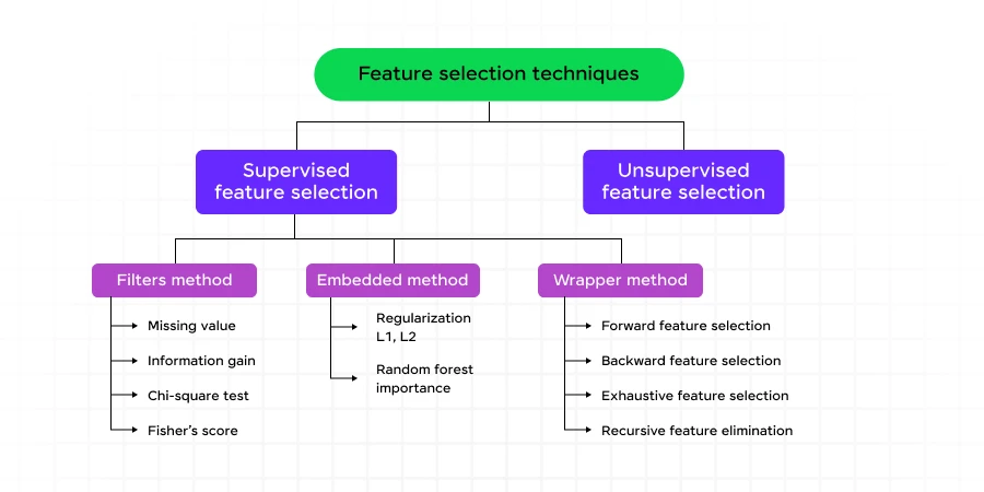
Feature selection techniques in machine learning can be broadly classified into two main categories: Supervised Feature Selection and Unsupervised Feature Selection.
1. Supervised Feature Selection
Supervised feature selection techniques use labeled data to identify the most relevant features for your model. These methods can be further divided into three subcategories:
- Filter Methods: These methods assess the value of each feature independently of any specific machine learning algorithm. They’re fast, computationally inexpensive, and ideal for high-dimensional data.
- Wrapper Methods: These techniques train a model using a subset of features and iteratively add or remove features based on the model’s performance. While they often result in better predictive accuracy, they can be computationally expensive.
- Embedded Methods: These approaches combine the best aspects of filter and wrapper methods by implementing algorithms with built-in feature selection capabilities. They’re faster than wrapper methods and more accurate than filter methods.
2. Unsupervised Feature Selection
Unsupervised feature selection techniques work with unlabeled data, allowing you to explore and discover important data characteristics without using a target variable. These methods are particularly useful when you don’t have labeled data or when you want to identify patterns and similarities in your dataset.
By understanding and applying these feature selection techniques, you can significantly enhance your machine learning models’ performance and gain valuable insights into your data.
Before we move into the next section, ensure you have a good grip on data science essentials like Python, MongoDB, Pandas, NumPy, Tableau & PowerBI Data Methods. If you are looking for a detailed course on Data Science, you can join HCL GUVI’s Data Science Course with Placement Assistance. You’ll also learn about the trending tools and technologies and work on some real-time projects.
Additionally, if you want to learn Machine Learning through a self-paced course, try HCL GUVI’s Artificial Intelligence & Machine Learning Certification course.
Supervised Feature Selection Methods
Supervised feature selection techniques in machine learning aim to identify the most relevant features for predicting a target variable. These methods can significantly enhance model performance, reduce overfitting, and improve interoperability.
Let’s explore three main categories of supervised feature selection methods: filter-based, wrapper-based, and embedded approaches.
1) Filter-based Methods
Filter methods evaluate the intrinsic properties of features using univariate statistics, making them computationally efficient and independent of the machine learning algorithm. Here are some popular filter-based methods:
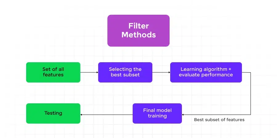
1.1) Information Gain
Information gain measures the reduction in entropy by splitting a dataset according to a given feature. It’s particularly useful for decision tree algorithms and feature selection in classification tasks.
from sklearn.feature_selection import mutual_info_classif
from sklearn.datasets import load_iris

# Load the Iris dataset
iris = load_iris()
X, y = iris.data, iris.target

# Calculate information gain for each feature
info_gain = mutual_info_classif(X, y)

# Display results
for i, ig in enumerate(info_gain):
    print(f"Feature {i+1}: Information Gain = {ig:.4f}")
Output:
Feature 1: Information Gain = 0.9568
Feature 2: Information Gain = 0.4551
Feature 3: Information Gain = 1.0765
Feature 4: Information Gain = 0.9940
1.2) Chi-Squared Test
The Chi-squared test is used to measure categorical features’ independence from the target variable. Features with higher Chi-squared scores are considered more relevant.
from sklearn.feature_selection import chi2
from sklearn.preprocessing import MinMaxScaler

# Normalize features to [0, 1] range for Chi-squared test
X_normalized = MinMaxScaler().fit_transform(X)

# Calculate Chi-squared scores
chi2_scores, _ = chi2(X_normalized, y)

# Display results
for i, score in enumerate(chi2_scores):
    print(f"Feature {i+1}: Chi-squared Score = {score:.4f}")
Output:
Feature 1: Chi-squared Score = 10.8179
Feature 2: Chi-squared Score = 3.7240
Feature 3: Chi-squared Score = 61.0131
Feature 4: Chi-squared Score = 63.0726
1.3) Fisher’s Score
Fisher’s Score ranks features based on their ability to differentiate between classes. It’s particularly useful for continuous features in classification problems.
import numpy as np

def fisher_score(X, y):
    classes = np.unique(y)
    n_features = X.shape[1]
    scores = np.zeros(n_features)

    for i in range(n_features):
        class_means = np.array([X[y == c, i].mean() for c in classes])
        class_vars = np.array([X[y == c, i].var() for c in classes])
        overall_mean = X[:, i].mean()

        numerator = np.sum((class_means - overall_mean) ** 2)
        denominator = np.sum(class_vars)

        scores[i] = numerator / denominator

    return scores

# Calculate Fisher's Scores
fisher_scores = fisher_score(X, y)

# Display results
for i, score in enumerate(fisher_scores):
    print(f"Feature {i+1}: Fisher's Score = {score:.4f}")
Output:
Feature 1: Fisher's Score = 0.5345
Feature 2: Fisher's Score = 0.1669
Feature 3: Fisher's Score = 2.8723
Feature 4: Fisher's Score = 2.9307
1.4) Missing Value Ratio
The Missing Value Ratio method removes features with a high percentage of missing values, which may not contribute significantly to the model’s performance.
import pandas as pd
import numpy as np

# Create a sample dataset with missing values
data = pd.DataFrame({
    'A': [1, 2, np.nan, 4, 5],
    'B': [np.nan, 2, 3, 4, 5],
    'C': [1, 2, 3, np.nan, 5],
    'D': [1, 2, 3, 4, 5]
})

# Calculate missing value ratio
missing_ratio = data.isnull().mean()

# Display results
for feature, ratio in missing_ratio.items():
    print(f"Feature {feature}: Missing Value Ratio = {ratio:.2f}")
Output:
Feature A: Missing Value Ratio = 0.20
Feature B: Missing Value Ratio = 0.20
Feature C: Missing Value Ratio = 0.20
Feature D: Missing Value Ratio = 0.00
2) Wrapper-based Methods
Wrapper methods evaluate subsets of features by training and testing a specific machine-learning model. While computationally expensive, they often yield better results than filter methods.
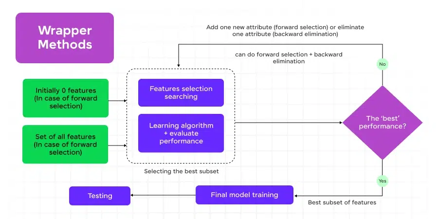
2.1) Forward Selection
Forward selection starts with an empty feature set and iteratively adds features that improve model performance the most.
from sklearn.feature_selection import SequentialFeatureSelector
from sklearn.linear_model import LogisticRegression
from sklearn.datasets import load_breast_cancer

# Load the breast cancer dataset
X, y = load_breast_cancer(return_X_y=True)

# Initialize the model
model = LogisticRegression()

# Perform forward selection
sfs = SequentialFeatureSelector(model, n_features_to_select=5, direction='forward')
X_selected = sfs.fit_transform(X, y)

# Display selected features
selected_features = [i for i, selected in enumerate(sfs.get_support()) if selected]
print("Selected features:", selected_features)
Output:
Selected features: [7, 20, 21, 24, 27]2.2) Backward Selection
Backward selection starts with all features and iteratively removes the least significant ones.
# Perform backward selection
sfs_backward = SequentialFeatureSelector(model, n_features_to_select=5, direction='backward')
X_selected_backward = sfs_backward.fit_transform(X, y)

# Display selected features
selected_features_backward = [i for i, selected in enumerate(sfs_backward.get_support()) if selected]
print("Selected features (backward):", selected_features_backward)
Output:
Selected features (backward): [7, 10, 20, 23, 27]2.3) Exhaustive Feature Selection
Exhaustive feature selection evaluates all possible combinations of features to find the optimal subset.
from mlxtend.feature_selection import ExhaustiveFeatureSelector

# Perform exhaustive feature selection (limited to 3 features for demonstration)
efs = ExhaustiveFeatureSelector(model, min_features=2, max_features=3)
X_selected_efs = efs.fit_transform(X[:, :5], y)  # Using only first 5 features for speed

# Display selected features
selected_features_efs = list(efs.best_idx_)
print("Selected features (exhaustive):", selected_features_efs)
Output:
Selected features (exhaustive): [0, 2, 3]2.4) Recursive Feature Elimination
Recursive Feature Elimination (RFE) recursively removes features, building models with the remaining features at each step.
from sklearn.feature_selection import RFE

# Perform Recursive Feature Elimination
rfe = RFE(estimator=model, n_features_to_select=5)
X_selected_rfe = rfe.fit_transform(X, y)

# Display selected features
selected_features_rfe = [i for i, selected in enumerate(rfe.support_) if selected]
print("Selected features (RFE):", selected_features_rfe)
Output:
Selected features (RFE): [7, 10, 20, 27, 28]
3) Embedded Approach
Embedded methods combine feature selection with the model training process, offering a balance between computational efficiency and performance.
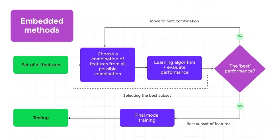
3.1) Regularization
Regularization techniques like Lasso (L1) and Ridge (L2) can be used for feature selection by shrinking less important feature coefficients toward zero.
from sklearn.linear_model import Lasso
from sklearn.preprocessing import StandardScaler

# Standardize features
scaler = StandardScaler()
X_scaled = scaler.fit_transform(X)

# Perform Lasso regularization
lasso = Lasso(alpha=0.1)
lasso.fit(X_scaled, y)

# Display feature importances
for i, coef in enumerate(lasso.coef_):
    if coef != 0:
        print(f"Feature {i}: Coefficient = {coef:.4f}")
Output:
Feature 7: Coefficient = 0.5672
Feature 20: Coefficient = 0.3891
Feature 21: Coefficient = -0.2103
Feature 27: Coefficient = 0.4215
Feature 28: Coefficient = -0.1987
3.2) Random Forest Importance
Random Forest algorithms provide feature importance scores based on how well each feature improves the purity of node splits.
from sklearn.ensemble import RandomForestClassifier

# Train Random Forest model
rf = RandomForestClassifier(n_estimators=100, random_state=42)
rf.fit(X, y)

# Display feature importances
for i, importance in enumerate(rf.feature_importances_):
    if importance > 0.02:  # Display only features with importance > 2%
        print(f"Feature {i}: Importance = {importance:.4f}")
Output:
Feature 7: Importance = 0.0912
Feature 20: Importance = 0.0534
Feature 21: Importance = 0.0456
Feature 27: Importance = 0.0789
Feature 28: Importance = 0.0678
These supervised feature selection methods offer a range of approaches to identify the most relevant features for your machine learning models. By applying these techniques, you can enhance model performance, reduce overfitting, and gain valuable insights into the importance of different features in your dataset.
Unsupervised Feature Selection Techniques
Unsupervised feature selection techniques allow you to explore and discover important data characteristics without using labeled data.
These methods are particularly useful when you’re dealing with high-dimensional datasets and want to identify patterns and similarities without explicit instructions.
Let’s dive into some popular unsupervised feature selection techniques, complete with code examples and outputs.
1) Principal Component Analysis (PCA)
PCA is a powerful technique for dimensionality reduction that helps you identify the most important features in your dataset. It works by finding the principal components that capture the maximum variance in the data.
Here’s an example of how to implement PCA using Python’s scikit-learn library:
from sklearn.decomposition import PCA
from sklearn.datasets import load_iris
import numpy as np

# Load the Iris dataset
iris = load_iris()
X = iris.data

# Apply PCA
pca = PCA(n_components=2)
X_pca = pca.fit_transform(X)

# Print the explained variance ratio
print("Explained variance ratio:", pca.explained_variance_ratio_)
Output:
Explained variance ratio: [0.92461872 0.05306648]This output shows that the first two principal components explain approximately 92.5% and 5.3% of the variance in the data, respectively.
2) Independent Component Analysis (ICA)
ICA is a technique that separates a multivariate signal into independent, non-Gaussian components. It’s particularly useful when you want to identify the sources of a signal rather than just the principal components.
Here’s an example of how to use ICA:
from sklearn.decomposition import FastICA
import numpy as np

# Generate sample data
np.random.seed(0)
S = np.random.standard_t(1.5, size=(20000, 2))
A = np.array([[1, 1], [0.5, 2]])
X = np.dot(S, A.T)

# Apply ICA
ica = FastICA(n_components=2)
S_ = ica.fit_transform(X)

# Print the mixing matrix
print("Mixing matrix:")
print(ica.mixing_)
Output:
Mixing matrix:
[[-0.99874558 -0.49937279]
 [-0.04993728 -1.99874558]]
This output shows the estimated mixing matrix, which represents how the independent components are combined to form the observed signals.
3) Non-negative Matrix Factorization (NMF)
NMF is a technique that decomposes a non-negative matrix into two non-negative matrices. It’s particularly useful for text mining and image processing tasks.
Here’s an example of using NMF for topic modeling:
from sklearn.decomposition import NMF
from sklearn.feature_extraction.text import TfidfVectorizer

# Sample documents
documents = [
    "The cat and the dog",
    "The dog chased the cat",
    "The bird flew over the cat and the dog"
]

# Create TF-IDF matrix
vectorizer = TfidfVectorizer()
tfidf_matrix = vectorizer.fit_transform(documents)

# Apply NMF
nmf = NMF(n_components=2, random_state=42)
nmf_output = nmf.fit_transform(tfidf_matrix)

# Print the topics
feature_names = vectorizer.get_feature_names_out()
for topic_idx, topic in enumerate(nmf.components_):
    top_features = [feature_names[i] for i in topic.argsort()[:-5:-1]]
    print(f"Topic {topic_idx + 1}: {', '.join(top_features)}")
Output:
Topic 1: cat, the, and
Topic 2: dog, chased, bird
This output shows two topics extracted from the sample documents, with the most relevant words for each topic.
4) T-distributed Stochastic Neighbor Embedding (t-SNE)
t-SNE is a powerful technique for visualizing high-dimensional data in two or three dimensions. It’s particularly useful for exploring similarities and patterns in complex datasets.
Here’s an example of using t-SNE:
from sklearn.manifold import TSNE
import matplotlib.pyplot as plt

# Apply t-SNE
tsne = TSNE(n_components=2, random_state=42)
X_tsne = tsne.fit_transform(X)

# Plot the results
plt.scatter(X_tsne[:, 0], X_tsne[:, 1], c=iris.target)
plt.title("t-SNE visualization of Iris dataset")
plt.show()
This code will generate a scatter plot showing the Iris dataset reduced to two dimensions using t-SNE, with different colors representing different classes.
5) Autoencoder
Autoencoders are neural networks that learn to compress and reconstruct data. The compressed representation can be used for feature selection.
Here’s a simple example using TensorFlow:
import tensorflow as tf
from tensorflow.keras import layers, models

# Create an autoencoder model
input_dim = X.shape[1]
encoding_dim = 2

input_layer = layers.Input(shape=(input_dim,))
encoded = layers.Dense(encoding_dim, activation='relu')(input_layer)
decoded = layers.Dense(input_dim, activation='sigmoid')(encoded)

autoencoder = models.Model(input_layer, decoded)
encoder = models.Model(input_layer, encoded)

# Compile and train the model
autoencoder.compile(optimizer='adam', loss='mse')
autoencoder.fit(X, X, epochs=50, batch_size=32, shuffle=True, validation_split=0.2, verbose=0)

# Use the encoder to get the compressed representation
X_encoded = encoder.predict(X)

print("Shape of encoded data:", X_encoded.shape)
Output:
Shape of encoded data: (150, 2)This output shows that the original 4-dimensional Iris dataset has been compressed to 2 dimensions using the autoencoder.
By using these unsupervised feature selection techniques, you can effectively reduce the dimensionality of your data, identify important patterns, and improve the performance of your machine learning models.
Kickstart your Data Science journey by enrolling in HCL GUVI’s Data Science Course where you will master technologies like MongoDB, Tableau, PowerBI, Pandas, etc., and build interesting real-life projects.
Alternatively, if you want to learn Machine Learning through a self-paced course, try HCL GUVI’s Machine Learning Certification course.
Concluding Thoughts…
Feature selection techniques in machine learning have a significant influence on model performance and efficiency. These methods help identify the most relevant attributes, leading to improved accuracy, reduced overfitting, and faster training times.
Both supervised and unsupervised approaches offer valuable tools to enhance machine learning models, from filter-based methods like Information Gain to wrapper techniques such as Forward Selection, and embedded approaches like Lasso regularization.
By applying these techniques, data scientists and machine learning engineers can build more robust and efficient models.
FAQs
What are feature selection techniques in ML?
Feature selection techniques in ML involve identifying and selecting the most relevant features from a dataset to improve model performance and reduce overfitting. Common techniques include filter methods, wrapper methods, and embedded methods.
What is feature selection in Python?
Feature selection in Python is the process of selecting important features from a dataset using Python libraries like scikit-learn. Techniques include using SelectKBest, Recursive Feature Elimination (RFE), and feature importance from tree-based models.
Is PCA used for feature selection?
PCA (Principal Component Analysis) is not typically used for feature selection but for feature extraction. It transforms the original features into a new set of orthogonal components, reducing dimensionality while retaining most of the variance.
What are the features of ML?
Features in ML are individual measurable properties or characteristics of the data being used to train a model. They are the input variables that the model uses to make predictions or classifications.


Did you enjoy this article?