Confusion Matrix in Machine Learning: The Ultimate Beginner’s Guide
Oct 03, 2025 5 Min Read 2753 Views
(Last Updated)
Machine learning is everywhere today, from chatbots, medical diagnosis, recommendation systems and even self-driving cars. But here’s a question: How can we be sure that these models are making the right predictions?
Accuracy alone isn’t enough. Consider a model that predicts all emails as “not spam.” It can have 90% accuracy, but it’s completely useless because it has missed all the actual spam emails.
This is why proper model evaluation is so important in data science. One of the easiest but most effective ways to evaluate a model is with a machine learning confusion matrix. A confusion matrix doesn’t just give you a right or wrong method for a prediction. It allows you to understand how well the model performed, what it got right, and where mistakes were made.
Here in this blog, we will break down the confusion matrix in ML in easy steps, study some real-world examples, and see how to read it for binary as well as multiclass classification problems. Whether you are a learner or refreshing data science basics, this article will help you get the clarity you need.
Table of contents
- What is the Confusion Matrix in Machine Learning?
- Structure of a Confusion Matrix
- Confusion Matrix Example in Machine Learning
- How to Interpret a Confusion Matrix in ML
- Accuracy
- Precision
- Recall (Sensitivity)
- F1-Score
- Confusion Matrix for Binary Classification
- Confusion Matrix in Python for Binary Classification
- Step 1: Import the Libraries
- Step 2: Define the Actual and Predicted Labels
- Step 3: Generate the Confusion Matrix
- Step 4: Visualize the Confusion Matrix
- Step 5: Classification Report
- Confusion Matrix for Multiclass Classification
- Confusion Matrix in Python for Multiclass Classification
- Step 1: Import the Libraries
- Step 2: Define the Actual and Predicted Labels
- Step 3: Compute the Confusion Matrix
- Step 4: Visualize the Confusion Matrix
- Step 5: Classification Report
- Confusion Matrix Advantages and Disadvantages
- Why the Confusion Matrix Matters in Data Science
- Final Thoughts..
- FAQs
- What is a confusion matrix in simple terms?
- Why do we need a confusion matrix when we already have accuracy?
- What is the difference between binary and multiclass confusion matrices?
- Which metrics can we calculate from a confusion matrix?
What is the Confusion Matrix in Machine Learning?
A confusion matrix in machine learning is a common method used for evaluating the performance of classification models. It is a tabular representation of actual targets and the model’s prediction that the model classifier produces.
Instead of just telling you the percentage of correct predictions, it highlights where your model is “confused.” That’s why it’s called a confusion matrix.
Structure of a Confusion Matrix
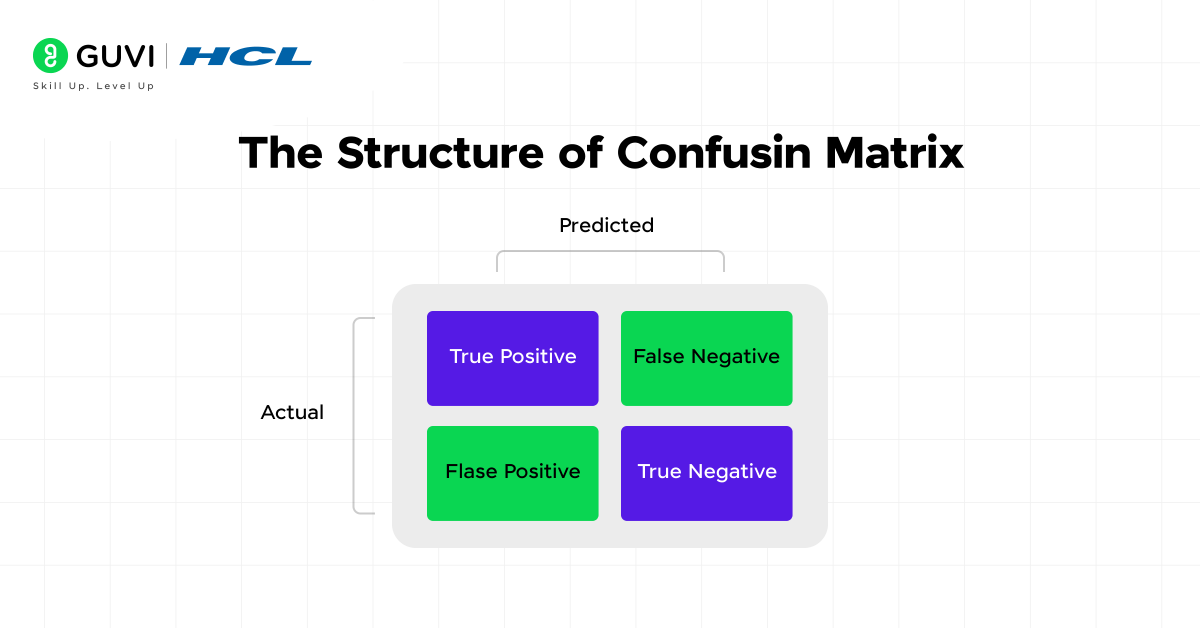
In a binary classification problem, it shows four possible outcomes at its core:

- True Positive (TP): The model said “Yes,” and it really was “Yes.”
- True Negative (TN): The model said “No,” and it really was “No.”
- False Positive (FP): The model said “Yes,” but it was really “No.” (Type I mistake)
- False Negative (FN): The model said “No,” but it was really “Yes.” (Type II mistake)
The term “confusion matrix” comes from the fact that it literally shows where the model is confused between different classes.
Confusion matrices aren’t new, they’ve been used in statistics since the 1960s, long before machine learning became popular.
A model can have 95% accuracy and still be terrible if the data is imbalanced (like predicting “not spam” every time). The confusion matrix helps you spot such hidden weaknesses.
Confusion Matrix Example in Machine Learning
Let’s imagine we built a spam email classifier:
| Predicted Spam | Predicted Not Spam | |
| Actual Spam | 85 (TP) | 15 (FN) |
| Actual Not Spam | 10 (FP) | 90 (TN) |
Here’s how to interpret it:
- The model properly found 85 spam emails (TP).
- It didn’t get 15 spam emails (FN).
- It wrongly identified 10 emails that weren’t spam as spam (FP).
- It properly identified 90 emails that weren’t spam (TN).
This table tells us far more than just overall accuracy; it shows where the model struggles.
How to Interpret a Confusion Matrix in ML
From the confusion matrix, we can calculate key performance metrics:
1. Accuracy
Accuracy is the overall percentage of correct predictions that a model makes. It is the ratio of how many predictions the model got correct to the total number of predictions that it makes. While accuracy can be helpful for an overall measure of performance, it can be a little misleading, especially with imbalanced data (data where one class appears much more frequently than the other). For example, when 95% of emails are “not spam”, a model that always predicts “not spam” will have 95% accuracy even if it never catches any spam emails.
Formula:

2. Precision
Precision tells us the quality of positive predictions. It answers the question: Of all the times the model predicted something as a positive, how many were actually correct? High precision indicates that there are fewer false positives. For example, If a medical test identified patients with a rare disease, precision tells us how many of the patients identified as “sick” were actually sick.
Formula:

3. Recall (Sensitivity)
Recall is the measure of a model’s ability to find all of the actual positives. Recall answers: Of all the positives in reality, how many did the model find? In other words, a model with high recall will not miss true cases. For example, In fraud detection, recall answers how many of the actual fraud transactions the system identified correctly.
Formula:

4. F1-Score
F1 score is a balance between precision and recall. Focusing only on precision or recall can sometimes be misleading. The F1 score helps bring both precision and recall together into a single number, which is useful especially in unbalanced data situations. The higher the F1 score, the better the model is in finding positives and lowering false positives.
Formula:

Confusion Matrix for Binary Classification
When we have only two classes (e.g., Spam vs. Not Spam, Fraud vs. Not Fraud, Positive vs. Negative), the confusion matrix is a 2×2 grid.
It looks like this:
| Predicted Positive | Predicted Negative | |
| Actual Positive | True Positive (TP) | False Negative (FN) |
| Actual Negative | False Positive (FP) | True Negative (TN) |
Example: Email Spam Detection
Suppose we have 100 emails:
- 50 are actually spam,
- 50 is not spam.
The model makes the following predictions:
| Predicted Spam | Predicted Not Spam | |
| Actual Spam | 45 (TP) | 5 (FN) |
| Actual Not Spam | 7 (FP) | 43 (TN) |
Interpretation:
- True Positives (45): Model correctly identified 45 spam emails.
- False Negatives (5): Model missed 5 spam emails (they slipped into the inbox).
- False Positives (7): Model marked 7 normal emails as spam.
- True Negatives (43): Model correctly identified 43 normal emails.
This simple 2×2 confusion matrix gives you an exact breakdown of where your binary classifier is performing well and where it’s making mistakes.
Confusion Matrix in Python for Binary Classification
Step 1: Import the Libraries
In Python, we’ll use NumPy for handling arrays, sklearn.metrics for generating the confusion matrix and classification report, and seaborn + matplotlib for visualization.
| import numpy as np import matplotlib.pyplot as plt import seaborn as sns from sklearn.metrics import confusion_matrix, classification_report |
Step 2: Define the Actual and Predicted Labels
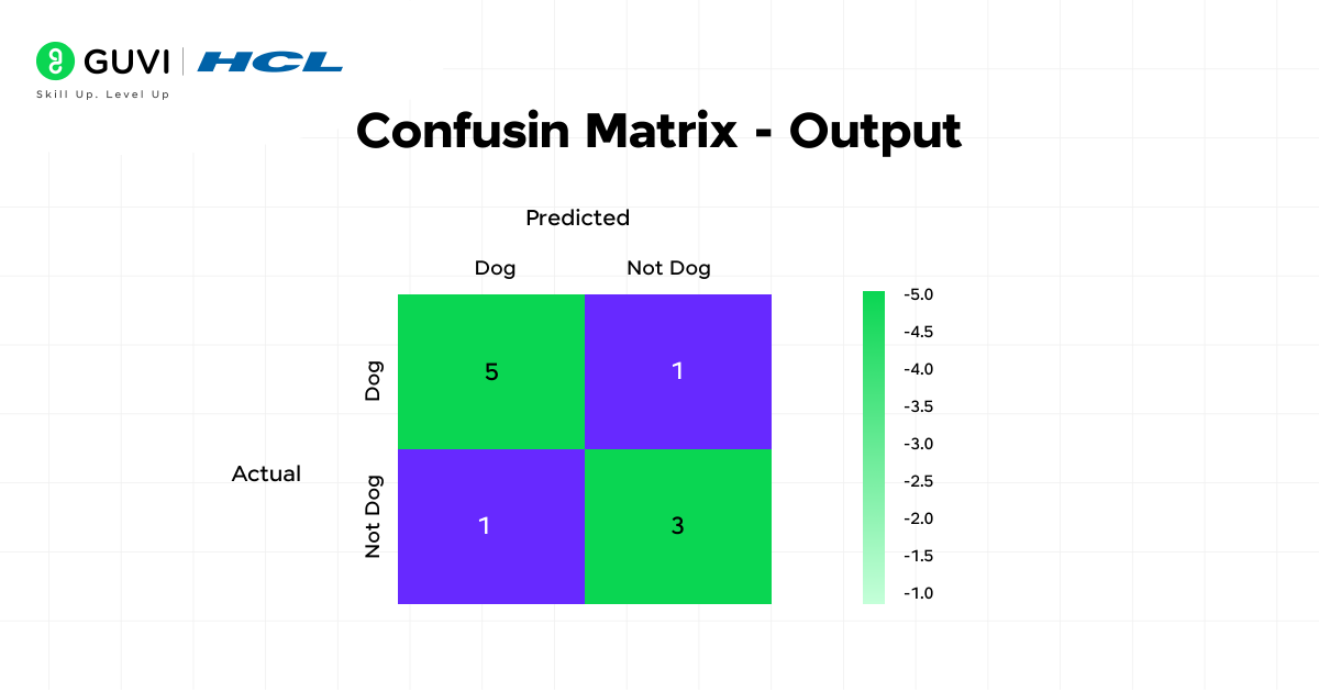
Imagine we are training a model to detect whether an image is of a Dog or not a dog.
| # Ground truth (what’s actually correct) true_labels = np.array([ ‘Dog’,’Dog’,’Dog’,’Not Dog’,’Dog’, ‘Not Dog’,’Dog’,’Dog’,’Not Dog’,’Not Dog’ ]) # Model predictions pred_labels = np.array([ ‘Dog’,’Not Dog’,’Dog’,’Not Dog’,’Dog’, ‘Dog’,’Dog’,’Dog’,’Not Dog’,’Not Dog’ ]) |
Step 3: Generate the Confusion Matrix
The confusion matrix compares actual labels with predicted labels.
| cm = confusion_matrix(true_labels, pred_labels) |
Step 4: Visualize the Confusion Matrix
We’ll use a heatmap to make it easy to interpret.
| plt.figure(figsize=(5,4)) sns.heatmap(cm, annot=True, fmt=’d’, cmap=”Blues”, xticklabels=[‘Dog’,’Not Dog’], yticklabels=[‘Dog’,’Not Dog’]) plt.ylabel(‘Actual’) plt.xlabel(‘Predicted’) plt.title(‘Confusion Matrix – Binary Classification’) plt.show() |

Step 5: Classification Report
Instead of manually calculating precision, recall, and F1-score, we can use classification_report.
| print(classification_report(true_labels, pred_labels)) |
Confusion Matrix for Multiclass Classification
Not all problems are binary. In many real-world cases, there are more than two categories. For example:
- Classifying handwritten digits (0–9).
- Identifying fruit types (apple, banana, orange).
- Predicting weather conditions (sunny, rainy, cloudy).
In such cases, the confusion matrix becomes an N×N table, where N is the number of classes. Each row represents the actual class, and each column represents the predicted class.
Example: Animal Classification
Let’s say we have a model that classifies animals into Cat, Dog, and Horse. After testing, we get this matrix:
| Predicted Cat | Predicted Dog | Predicted Horse | |
| Actual Cat | 40 | 8 | 2 |
| Actual Dog | 5 | 50 | 5 |
| Actual Horse | 3 | 4 | 43 |
Interpretation:
- Out of 50 actual Cats, the model predicted 40 correctly but confused 8 as Dogs and 2 as Horses.
- Out of 60 actual Dogs, the model got 50 right but confused 5 as Cats and 5 as Horses.
- Out of 50 actual Horses, it predicted 43 correctly but mislabeled 7 as either Cats or Dogs.
This helps us figure out where the model isn’t working. In this example, it sometimes mixes Cats with Dogs, which could mean that the traits of these two groups are similar.
Confusion Matrix in Python for Multiclass Classification
Step 1: Import the Libraries
(Same as before, but let’s keep it clear for students.)
| import numpy as np import matplotlib.pyplot as plt import seaborn as sns from sklearn.metrics import confusion_matrix, classification_report |
Step 2: Define the Actual and Predicted Labels
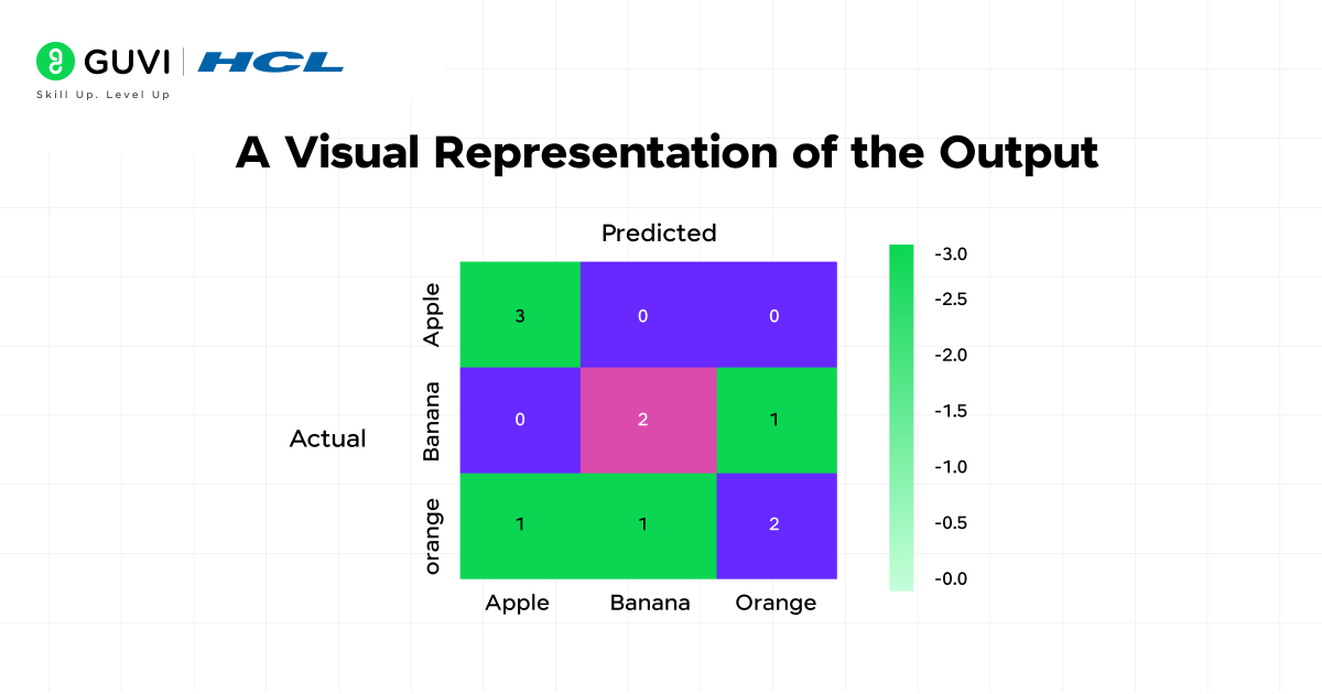
Here, the true labels are what the fruits really are, while the predicted labels are what our model thinks they are.
| # Ground truth (actual fruits) true_labels = np.array([ ‘Apple’,’Banana’,’Orange’,’Apple’,’Orange’, ‘Banana’,’Apple’,’Orange’,’Orange’,’Banana’ ]) # Model predictions pred_labels = np.array([ ‘Apple’,’Orange’,’Orange’,’Apple’,’Banana’, ‘Banana’,’Apple’,’Orange’,’Apple’,’Banana’ ]) |
Step 3: Compute the Confusion Matrix
| cm = confusion_matrix(true_labels, pred_labels, labels=[‘Apple’,’Banana’,’Orange’]) |
Step 4: Visualize the Confusion Matrix
A heatmap makes it easy to see where the model is doing well and where it’s confusing one fruit with another.
| cm = confusion_matrix(true_labels, pred_labels, labels=[‘Apple’,’Banana’,’Orange’]) plt.figure(figsize=(6,5)) sns.heatmap(cm, annot=True, fmt=’d’, cmap=”Oranges”, xticklabels=[‘Apple’,’Banana’,’Orange’], yticklabels=[‘Apple’,’Banana’,’Orange’]) plt.ylabel(‘Actual’) plt.xlabel(‘Predicted’) plt.title(‘Confusion Matrix – Multiclass Classification’) plt.show() |

Step 5: Classification Report
| print(classification_report(true_labels, pred_labels)) |
This gives a detailed summary for each class separately (precision, recall, F1-score), unlike binary classification where it’s just two.
Confusion Matrix Advantages and Disadvantages
| Advantages | Disadvantages |
| Provides a detailed breakdown of classification results. | Can become complex to interpret for many classes. |
| Helps identify specific types of errors (False Positives vs False Negatives). | Doesn’t directly show overall performance in one number. |
| Useful for imbalanced datasets where accuracy is misleading. | Needs additional metrics like Precision, Recall, and F1-score for complete evaluation. |
| Works for both binary and multiclass classification. | May overwhelm beginners when too many classes are involved. |
Why the Confusion Matrix Matters in Data Science
In practical data science projects, simply knowing that your model is “80% accurate” doesn’t mean much. Take a fraud detection model in which only 1 in 100 transactions is fraudulent. If your model predicts “No fraud” every time, you will be 99% accurate, which is useless.
The confusion matrix in classification allows you to get the complete story. It helps you identify whether your model is really learning patterns or just taking shortcuts.
Now that you know how the Confusion Matrix works, why stop here? Take your next step with HCL GUVI’s Advanced AI & Machine Learning Course, designed in collaboration with Intel and IITM Pravartak. This program takes you from theory to hands-on projects and real-world applications in Python, ML algorithms, Deep Learning, NLP, and model deployment.
Highlights of the Program:
- Intel-certified credential recognized globally
- Learn from industry experts and IITM Pravartak faculty
- Real-world case studies and hands-on projects
- Flexible learning with mentor support & career guidance
Final Thoughts..
In machine learning, the confusion matrix is more than just a table: it’s a view into your model’s advantages and limitations. The confusion matrix is your reference point for good data model evaluation, whether you’re dealing with binary classification, multiclass classification, calculating precision and recall or aspects related to confusion matrices.
If you’re learning about confusion matrix in Python using scikit-learn, start small with a binary example, and then build up to multiclass problems.
I hope this blog helped you understand what a confusion matrix in machine learning is and how to use it for binary and multiclass classification problems. Remember, learning machine learning concepts takes a lot of practice, so don’t worry if you feel stuck initially, you’ll be able to improve each time you complete a project.
FAQs
1. What is a confusion matrix in simple terms?
A confusion matrix is a table that indicates how well a machine learning model performed by showing the difference between actual and predicted values.
2. Why do we need a confusion matrix when we already have accuracy?
Accuracy simply tells you the overall percentage of correct predictions whereas a confusion matrix provides more detail as to the exact types of the errors (i.e., false positives or false negatives).
3. What is the difference between binary and multiclass confusion matrices?
In the case of binary classification, a confusion matrix is 2×2 and is used for binary classification problems where there are two outcomes (e.g., spam vs. not spam).
In the case of multiclass classification, the confusion matrix is larger (3×3, 4×4, etc.) depending on how many classes there are.
4. Which metrics can we calculate from a confusion matrix?
From a confusion matrix we can compute accuracy, precision, recall, and F1-score


Did you enjoy this article?