What is DBSCAN Clustering in Machine Learning?
Oct 22, 2025 7 Min Read 2575 Views
(Last Updated)
What if your dataset forms patterns that do not look like neat circles or balanced groups? In such cases, conventional algorithms like K-Means often fail, but DBSCAN deals with these challenges by grouping points through density and leaving isolated points as noise. This ability makes it highly effective for messy and irregular real-world data.
In this blog, you will explore how DBSCAN works, the parameters that guide it, its advantages, its applications, its limitations, and a step-by-step Python implementation to see it in action.
Table of contents
- What is DBSCAN Clustering?
- Key Parameters in DBSCAN
- eps (Epsilon)
- minPts (Minimum Points)
- Relationship Between eps and minPts
- How Does DBSCAN Work?
- Implementation of DBSCAN Algorithm in Python
- Step 1: Import Libraries
- Step 2: Generate the Dataset
- Step 3: Apply DBSCAN with Different Parameters
- Step 4: Visualize the Clusters
- Step 5: Evaluate the Results
- Top Benefits of DBSCAN
- No Need to Specify Clusters
- Proficiency to Handle Irregular Shapes
- Effective Noise Handling
- Adaptability to Different Densities
- Applications of DBSCAN Clustering
- Anomaly Detection
- Geospatial Analysis
- Image and Signal Processing
- Biological and Medical Research
- Limitations of DBSCAN Clustering
- Sensitivity to Parameter Selection
- Difficulty with High-Dimensional Data
- Struggles with Varying Densities
- Computational Cost for Large Datasets
- K-Means versus DBSCAN Clustering
- Quick Quiz on DBSCAN Clustering
- Q1. Which type of points does DBSCAN classify as noise?
- Q2. Which parameter defines the neighborhood radius in DBSCAN?
- Q3. What happens if eps is too large?
- Q4. In DBSCAN, what does a label of -1 represent?
- Q5. Which task is DBSCAN especially suited for?
- Conclusion
- FAQs
- Is DBSCAN suitable for very large datasets?
- How is DBSCAN different from hierarchical clustering?
- Can DBSCAN be combined with other techniques?
What is DBSCAN Clustering?
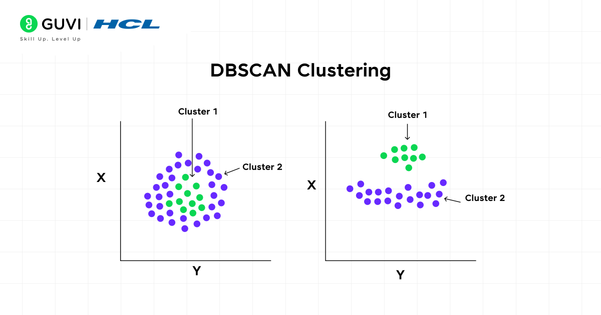
DBSCAN (Density-Based Spatial Clustering of Applications with Noise) is an unsupervised machine learning algorithm. It is used for clustering data points based on their density. DBSCAN is distinct from conventional methods such as k-means as it does not require the number of clusters to be specified in advance. Instead, it groups together points that are closely packed (high-density regions) and marks points that lie alone in low-density regions as outliers or noise.
Key Parameters in DBSCAN
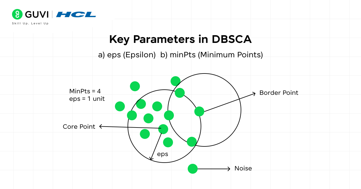
DBSCAN clustering in machine learning relies on two important parameters that guide how clusters are identified:
1. eps (Epsilon)
Represents the maximum distance between two points so they can be considered neighbors. Two points p and q are neighbors if the distance dist(p, q) ≤ eps. A smaller value of eps may split a cluster into multiple groups. A larger value may merge separate clusters into one.
2. minPts (Minimum Points)
Refers to the minimum number of points required to form a dense region. A point p is classified as a core point if the number of neighbors within eps satisfies |N(p)| ≥ minPts, where N(p) is the neighborhood of p. A higher value of minPts makes the algorithm stricter, while a lower value may lead to smaller clusters.
Note: For most cases, a minimum value of minPts = 3 is recommended, although larger datasets often use higher values to improve reliability.
Relationship Between eps and minPts
These parameters work together to decide whether data points form clusters or remain as noise. A cluster forms when at least one core point has minPts neighbors within eps, and these points are connected through density reachability. A poor choice of eps and minPts can lead to over-clustering or under-clustering, which makes the results less meaningful.
How Does DBSCAN Work?
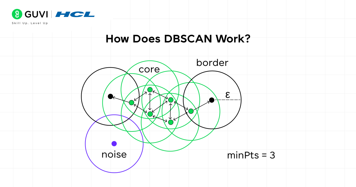
The working of DBSCAN clustering in ML can be explained through the classification of points into three categories:
- Core Points: A point is called a core point if it has at least minPts neighbors within the distance eps. These points represent dense regions that help form clusters.
- Border Points: A point is called a border point if it falls within the neighborhood of a core point but does not have enough neighbors to be a core point itself. Border points belong to a cluster, but they do not expand it further.
- Noise Points: A point is treated as noise if it is neither a core point nor a border point. Such points are considered outliers and remain outside clusters.
The process starts with an unvisited point. If this point qualifies as a core point, a new cluster begins. All points within the eps neighborhood are added to this cluster. Any neighbor that is also a core point expands the cluster further by including its own neighbors. Border points are attached to the nearest core point cluster. Noise points remain unassigned because they lack sufficient density. This process continues until all points are visited and assigned appropriately.
Implementation of DBSCAN Algorithm in Python
DBSCAN is available in the scikit-learn library and can be demonstrated with a synthetic dataset. The process includes creating data, applying DBSCAN, visualizing clusters, and evaluating results.
Step 1: Import Libraries
We start by importing the essential libraries for clustering, visualization, and evaluation.
import numpy as np
import matplotlib.pyplot as plt
from sklearn.cluster import DBSCAN
from sklearn.datasets import make_blobs
from sklearn import metrics
from sklearn.metrics import adjusted_rand_score
Step 2: Generate the Dataset
A dataset of 300 points grouped into four clusters is created with make_blobs.
X, y_true = make_blobs(n_samples=300, centers=4,
cluster_std=0.50, random_state=42)
This dataset has four natural groups that will allow us to test how DBSCAN behaves under different parameter values.
Also, read: Top 11 Python Libraries For Machine Learning in 2025
Step 3: Apply DBSCAN with Different Parameters
Case A: eps = 0.2, min_samples = 5
A small neighborhood radius (eps=0.2) with fewer points required to form a cluster (min_samples=5).
db1 = DBSCAN(eps=0.2, min_samples=5).fit(X)
labels1 = db1.labels_
Case B: eps = 0.5, min_samples = 5
A larger radius (eps=0.5) with the same minimum points.
db2 = DBSCAN(eps=0.5, min_samples=5).fit(X)
labels2 = db2.labels_
Case C: eps = 0.5, min_samples = 15
The same radius as Case B, but with more points required to form a dense region.
db3 = DBSCAN(eps=0.5, min_samples=15).fit(X)
labels3 = db3.labels_
Step 4: Visualize the Clusters
We can plot each case side by side to see how clusters change.
fig, axes = plt.subplots(1, 3, figsize=(15, 4))
for ax, labels, title in zip(
axes, [labels1, labels2, labels3],
[“eps=0.2, min_samples=5”, “eps=0.5, min_samples=5”, “eps=0.5, min_samples=15”]):
unique_labels = set(labels)
colors = plt.cm.Spectral(np.linspace(0, 1, len(unique_labels)))
for k, col in zip(unique_labels, colors):
if k == -1:
col = ‘k’ # noise in black
class_member_mask = (labels == k)
xy = X[class_member_mask]
ax.plot(xy[:, 0], xy[:, 1], ‘o’,
markerfacecolor=col, markeredgecolor=’k’, markersize=6)
ax.set_title(title)
plt.show()
- In Case A, the small radius causes many points to be marked as noise.
- In Case B, clusters form clearly with fewer noise points.
- In Case C, requiring more neighbors leads to some points being rejected as noise even inside clusters.
Step 5: Evaluate the Results
Silhouette Score and Adjusted Rand Index (ARI) help compare the three cases.
print(“Case A”)
print(“Silhouette Score:”, metrics.silhouette_score(X, labels1))
print(“ARI:”, adjusted_rand_score(y_true, labels1))
print(“\nCase B”)
print(“Silhouette Score:”, metrics.silhouette_score(X, labels2))
print(“ARI:”, adjusted_rand_score(y_true, labels2))
print(“\nCase C”)
print(“Silhouette Score:”, metrics.silhouette_score(X, labels3))
print(“ARI:”, adjusted_rand_score(y_true, labels3))
Sample Output:
Case A
Silhouette Score: 0.05
ARI: 0.22
Case B
Silhouette Score: 0.46
ARI: 0.81
Case C
Silhouette Score: 0.39
ARI: 0.74
The results show that Case B produces the best clustering for this dataset. Case A is too strict, leading to too many noise points. Case C weakens the cluster quality by rejecting valid points as noise.
Master the art of clustering and advanced machine learning techniques with our Artificial Intelligence and Machine Learning Course. powered by Intel Certification. This comprehensive course takes you from the foundations of supervised and unsupervised learning (including DBSCAN and other clustering methods) to deep learning, MLOps, and real-world applications. With personalized mentorship and placement support, you’ll not only learn theory but also gain the practical AI expertise employers are looking for. Enroll now and validate your skills with Intel Certification to accelerate your AI career.
Top Benefits of DBSCAN
1. No Need to Specify Clusters
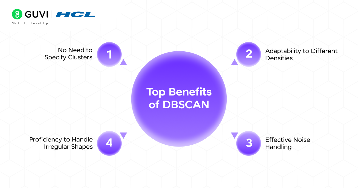
DBSCAN does not require the number of clusters to be chosen before running the algorithm. The clusters are formed automatically according to the density of data points. This saves time and reduces the risk of forcing the dataset into an artificial structure.
2. Proficiency to Handle Irregular Shapes
Clusters in many datasets are not spherical. DBSCAN adapts to curved and uneven groups because it relies on density rather than distance from centroids. This makes the algorithm suitable for spatial and scientific data where natural shapes are rarely uniform.
3. Effective Noise Handling
Many clustering methods force every data point into a cluster. DBSCAN clustering treats low-density points as noise, which helps protect the structure of genuine clusters. These outliers remain outside the main groups, which gives cleaner and more meaningful results.
4. Adaptability to Different Densities
DBSCAN clustering can capture both dense and sparse clusters within the same dataset. This flexibility allows the algorithm to reveal hidden structures that traditional methods may miss. It is especially valuable in data where groups vary in size and distribution.
Applications of DBSCAN Clustering
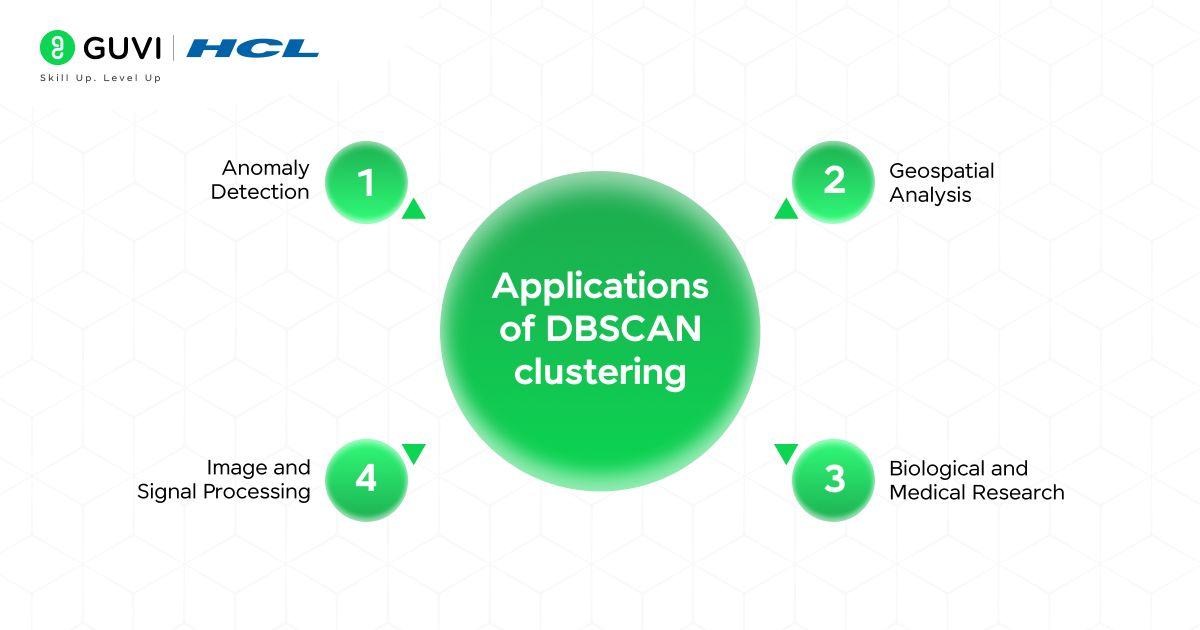
DBSCAN is widely used in fields where data contains irregular patterns and noise. Here are some common use cases:
1. Anomaly Detection
DBSCAN identifies dense areas of activity and separates them from scattered points, which makes it reliable for detecting anomalies. In banking, clusters of legitimate transactions form naturally, while fraudulent attempts are isolated as noise.
In network security, traffic that follows expected patterns falls into well-defined clusters, while irregular flows remain outside. In sensor-based systems, faulty readings that do not match the density of other data are automatically flagged.
2. Geospatial Analysis
Irregular shapes in real-world data require an algorithm that does not assume clusters are spherical. DBSCAN adapts to this challenge by grouping points that are close together while leaving distant ones aside. In mapping applications, nearby restaurants, hospitals, and shops are grouped into clusters that reflect busy urban zones, while remote locations stand apart.
In transportation studies, DBSCAN highlights high-density vehicle movement across main routes, while quieter roads are separated. City planners use the same approach to identify concentrated areas of housing or commerce, which helps in designing infrastructure.
3. Image and Signal Processing
Noise handling is one of the strongest features of DBSCAN, which makes it well-suited for images and signals. In image segmentation, regions of pixels with similar intensity form meaningful clusters, while scattered pixels that do not belong are ignored.
Medical imaging benefits similarly, as dense tissue structures can be separated from surrounding areas that lack consistency. Signal processing also relies on DBSCAN to identify recurring frequency patterns while leaving random disturbances outside clusters.
4. Biological and Medical Research
Biological data often contains irregular and uneven groups, and DBSCAN adapts well to such complexity. In gene expression studies, clusters of genes with similar behavior emerge naturally, while rare gene activity appears as noise. Protein structures show similar irregular densities, which DBSCAN can capture without needing predefined shapes.
Medical imaging provides another case where dense areas that may represent tumors are separated from normal regions, giving doctors and researchers clearer insights. The flexibility to handle uneven densities and irregular structures makes DBSCAN an important tool in biological and medical research.
Also, Read: The Machine Learning Cheat Sheet [2025 Guide]
Limitations of DBSCAN Clustering
1. Sensitivity to Parameter Selection
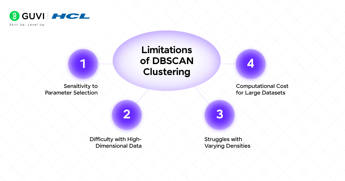
The quality of clustering depends strongly on the choice of eps and minPts. A small value of eps can break one cluster into many parts, while a large value can merge distinct clusters. Similarly, an unsuitable minPts value can either create scattered clusters or reject valid points as noise. Parameter tuning is therefore critical and sometimes difficult for complex datasets.
2. Difficulty with High-Dimensional Data
DBSCAN does not scale well with high-dimensional data because distance measures lose meaning as dimensions increase. This issue, known as the curse of dimensionality, leads to poor cluster separation. Applications such as text embeddings or genomic data often require dimensionality reduction techniques before DBSCAN can be applied effectively.
3. Struggles with Varying Densities
DBSCAN assumes one global eps value for the entire dataset. When clusters vary in density, a single eps cannot fit both dense and sparse regions. As a result, dense clusters may be identified correctly, but sparser ones may be labeled as noise or left incomplete.
4. Computational Cost for Large Datasets
The algorithm calculates distances between points, which becomes expensive with very large datasets. Processing millions of records in the basic form of DBSCAN can be slow. More advanced versions with indexing structures or parallelization are often required to make DBSCAN efficient at scale.
K-Means versus DBSCAN Clustering
Both K-Means and DBSCAN clustering are clustering algorithms, but they differ in how they define clusters and how they handle real-world data challenges. The table below provides a detailed comparison:
| Key Factor | K-Means | DBSCAN |
| Cluster Definition | Uses distance from centroids to form clusters | More effective on low to medium-dimensional data, may struggle as dimensions increase |
| Number of Clusters | Must be chosen before running the algorithm | Determined automatically through eps and minPts |
| Cluster Shape | Works well when clusters are spherical or evenly distributed | Captures clusters of irregular shapes and varying densities |
| Noise and Outliers | Every point is forced into a cluster, even outliers | Outliers are labeled as noise and remain outside clusters |
| Data Requirements | Performs well with balanced data where clusters are similar in size | Performs well with unbalanced data and can separate dense regions from sparse ones |
| Scalability | Efficient on very large datasets and high-dimensional data | Results depend on the correct selection of eps and minPts |
| Sensitivity | Results depend on centroid initialization and are strongly affected by outliers | Results depend on correct selection of eps and minPts |
| Use Cases | Market basket analysis and image compression | Geospatial clustering and separating noise from meaningful patterns |
Quick Quiz on DBSCAN Clustering
Q1. Which type of points does DBSCAN classify as noise?
a) Core points
b) Border points
c) Points without enough neighbors
d) All points in dense clusters
Q2. Which parameter defines the neighborhood radius in DBSCAN?
a) minPts
b) eps
c) silhouette
d) centroid
Q3. What happens if eps is too large?
a) Clusters split into smaller groups
b) Clusters merge together
c) More points are labeled as noise
d) No clusters are formed
Q4. In DBSCAN, what does a label of -1 represent?
a) A core point
b) A border point
c) A noise point
d) A cluster with low density
Q5. Which task is DBSCAN especially suited for?
a) Finding centroids in balanced datasets
b) Grouping points into spherical clusters
c) Identifying irregular clusters and outliers
d) Compressing image data into pixels
Answers:
- c) Points without enough neighbors
- b) eps
- b) Clusters merge
- c) A noise point
- c) Identifying irregular clusters and outliers
Conclusion
DBSCAN clustering stands out as a clustering algorithm because it identifies groups of data points based on density and separates noise without forcing every point into a cluster. It handles irregular shapes better than many traditional methods and offers flexibility for real-world datasets. With the right approach, DBSCAN becomes a reliable choice for tasks such as anomaly detection and scientific research. Experiment with different parameters and compare results with other clustering methods, then decide where DBSCAN delivers the best fit for your problem.
FAQs
1. Is DBSCAN suitable for very large datasets?
DBSCAN can handle medium to large datasets, but performance slows down as the number of points increases. Distance calculations become expensive, and processing millions of rows requires optimized versions such as parallel DBSCAN or GPU-accelerated implementations.
2. How is DBSCAN different from hierarchical clustering?
Hierarchical clustering builds a tree of clusters step by step, while DBSCAN groups points based on density in one pass. Hierarchical methods often require deciding a cut-off point in the tree, but DBSCAN automatically separates dense regions and marks noise without such decisions.
3. Can DBSCAN be combined with other techniques?
DBSCAN is often used with preprocessing methods like PCA or t-SNE for dimensionality reduction. It can also be paired with supervised learning where DBSCAN first labels data into clusters, and those labels are then used as features for classification or regression.





Did you enjoy this article?