Understanding Complexity Analysis in Data Structures: A Beginner’s Guide

Ever wondered why some programs run instantly while others slow to a crawl with just a little more data? The secret often lies in something called complexity analysis. If you’re just stepping into the world of data structures and algorithms, understanding how your code performs as the input size grows is a skill that separates a beginner from a thoughtful problem solver.

So, what exactly is complexity analysis in data structures, and why should you care? Let us learn more about that in this article!

What is Complexity Analysis in Data Structures?

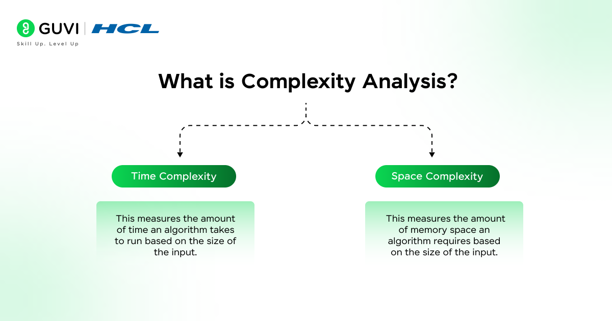
Complexity analysis in data structures is the process of determining how the performance of an algorithm changes with the size of the input. In other words, it helps us evaluate the efficiency of an algorithm in terms of time and space. As a beginner, it’s important to focus on the two primary types of complexity:

1. Time Complexity: This measures the amount of time an algorithm takes to run based on the size of the input.
2. Space Complexity: This measures the amount of memory space an algorithm requires based on the size of the input.

Why is Complexity Analysis Important?

In the real world, we deal with large datasets. Some algorithms might work just fine for small datasets, but could become extremely slow or inefficient when scaled up. By analyzing the complexity, we can choose the right data structure and algorithm that ensures our programs perform well, even with large inputs.

Big O Notation

The most commonly used way to express complexity is through Big O notation. It describes the upper bound of the algorithm’s running time or memory usage in the worst-case scenario. It provides a high-level understanding of how the algorithm behaves as the input size grows.

Here are some key time complexities you’ll encounter in your studies:

1. O(1) – Constant Time:
   An algorithm is said to have constant time complexity if it takes the same amount of time to execute, regardless of the input size. For example, accessing an element in an array by index takes constant time, i.e., O(1).
   
2. O(log n) – Logarithmic Time:
   Logarithmic time complexity arises in algorithms that reduce the problem size by half with each step. Binary search is a classic example where the problem size gets halved each time, making it very efficient compared to linear search.
   
3. O(n) – Linear Time:
   If an algorithm’s running time increases linearly with the input size, it has O(n) complexity. For example, if you iterate over all elements of an array once, the time complexity is O(n).
   
4. O(n log n) – Linearithmic Time:
   This complexity is common in algorithms that divide the input into smaller chunks and process them, like Merge Sort and Quick Sort. These algorithms are more efficient than O(n^2) but still not as fast as O(log n).
   
5. O(n^2) – Quadratic Time:
   Algorithms with quadratic time complexity are typically nested loops, where the time grows exponentially as the input size increases. For example, bubble sort or selection sort have O(n^2) complexity, meaning that as the input size grows, the time taken grows significantly.
   
6. O(2^n) – Exponential Time:
   Exponential time complexity is very inefficient and occurs in algorithms that solve problems by brute force. For example, many recursive algorithms may have this complexity, like the Fibonacci sequence (without memoization).

What is Space Complexity?

While time complexity focuses on the runtime, space complexity analyzes the amount of memory needed. Here are a few common scenarios:

• O(1) – Constant Space: The algorithm uses a fixed amount of space, regardless of input size.
• O(n) – Linear Space: The algorithm uses memory proportional to the size of the input.

For example, a simple sorting algorithm like bubble sort has O(1) space complexity because it sorts the array in place without using extra memory. However, a divide-and-conquer algorithm like merge sort requires additional space to store the subarrays, resulting in O(n) space complexity.

Analyzing Common Data Structures

Let’s look at how complexity analysis applies to common data structures.

• Arrays:
  
  • Accessing an element: O(1)
    
  • Inserting at the end: O(1)
    
  • Inserting at the beginning: O(n)
    
  • Searching: O(n)
    
• Linked Lists:
  
  • Accessing an element: O(n)
    
  • Inserting at the beginning: O(1)
    
  • Deleting a node: O(1) (if we have direct access to the node)
    
  • Searching: O(n)
    
• Stacks and Queues:
  Both have O(1) time complexity for common operations like push, pop, and enqueue because these operations are done at one end (top/front).
  
• Hash Tables:
  
  • Insert, delete, and search: O(1) on average, though collisions can cause performance degradation.
    
• Trees (e.g., Binary Search Tree):
  
  • Search, insertion, deletion: O(log n) in balanced trees, but can degrade to O(n) if the tree is unbalanced.

Practical Example: Sorting Algorithms

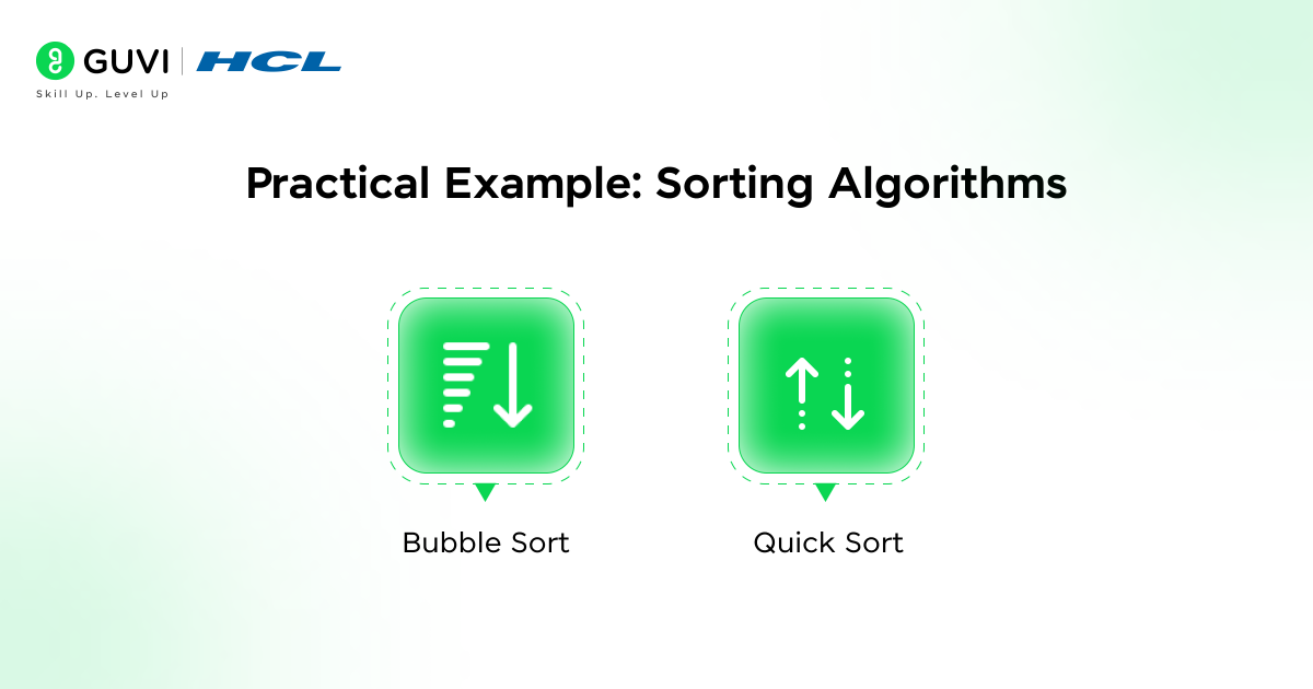
Let’s look at a simple example of how time complexity plays out in sorting algorithms.

• Bubble Sort:
  Bubble sort compares adjacent elements and swaps them if they are in the wrong order. It goes through the entire list repeatedly, which results in O(n^2) time complexity.
  
• Quick Sort:
  Quick sort uses the divide-and-conquer approach, splitting the array into two subarrays and recursively sorting them. On average, its time complexity is O(n log n), making it much faster than bubble sort for large datasets.
  

So, after reading all this, if you are ready to start your journey in learning Data Structures and Algorithms, consider enrolling in GUVI’s Data Structures and Algorithms Course with Python – IIT-M Pravartak Certified which includes four in-depth courses across Python, Java, C, and JavaScript. It also helps you to master algorithmic problem-solving and prepare for technical interviews with industry-grade certification!

Conclusion

Understanding complexity analysis helps us make better decisions about which algorithms and data structures to use in different scenarios. As a beginner, mastering these concepts will significantly improve your ability to design efficient programs. You can start by analyzing simple algorithms and data structures, gradually moving to more complex ones as you gain experience.

Remember, the goal is not always to find the most complex algorithm, but the one that strikes the right balance between efficiency and simplicity for your specific problem.