Binary Trees in Data Structure: A Comprehensive Guide
Oct 23, 2025 8 Min Read 1961 Views
(Last Updated)
Why do so many data structures, maps, heaps, syntax trees, and priority queues all trace back to one foundational idea: the binary tree?
If you’ve ever wondered how computers organize information in a way that lets them search, decide, prioritize, or evaluate with remarkable efficiency, binary trees are the hidden architecture behind the scenes.
In this article, we’ll explore what binary trees really are, why shapes like BSTs and heaps exist, how operations like search and traversal work, where balancing comes into play, and how these trees show up in real-world systems you use every day. So, let’s get started!
Table of contents
- What are Binary Trees?
- Why Should You Care About Binary Trees?
- Types of Binary Trees
- Full (or Strict) Binary Tree
- Perfect Binary Tree
- Complete Binary Tree
- Skewed (Degenerate) Binary Tree
- Balanced Binary Tree
- Binary Search Tree (BST)
- Heap (Min or Max)
- Expression Tree
- Core Operations & Algorithms
- Search
- Deletion
- Traversals – “How do we walk the tree?”
- Height & Balance Check
- Use Cases & Applications
- Ordered data structures
- Priority queues and scheduling
- Compilers and interpreters
- Compression and networking
- Decision-making and games
- Implementation Tips & Pitfalls
- Conclusion
- FAQs
- What is the difference between a Binary Tree and a Binary Search Tree?
- Why do we use binary trees in data structures?
- What are the types of binary trees?
- What are common operations on a BST?
- What happens if a BST becomes unbalanced?
What are Binary Trees?
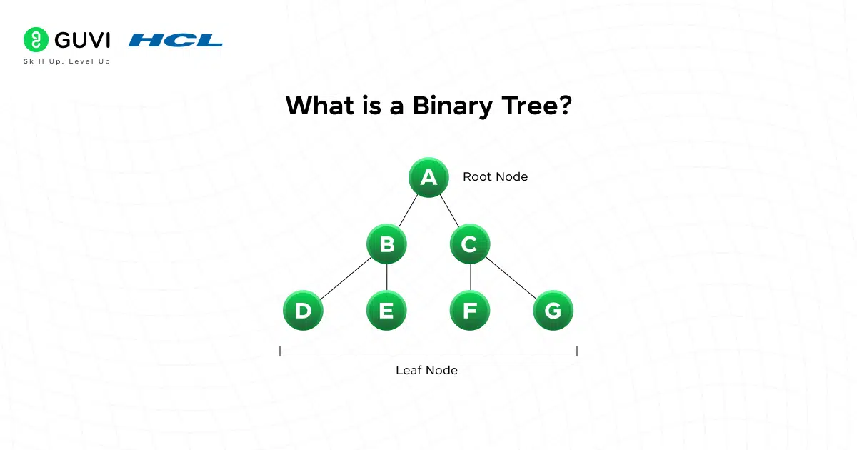
At its core, a binary tree is a hierarchical data structure in which each node has at most two children: usually called the left child and the right child.
You can think of it like a family tree, but each person (node) can have up to two children, not many more. Because of that constraint, binary trees offer efficiency and structure, letting you perform many operations (search, insert, delete, traverse) in ways that are easier to control.
Here’s the language we use when working with binary trees:
| Term | What it means |
| Node | A box of data + links to children |
| Root | The top-most node |
| Parent | Node above |
| Child | Node below |
| Leaf | Node with no children |
| Internal Node | Node with 1 or 2 children |
| Subtree | A node and everything under it |
| Depth | Levels from root to a node |
| Height | Longest path from a node to a leaf (root height = tree height) |
Understanding height is crucial in binary trees because many time complexities depend on it.
Why Should You Care About Binary Trees?
Let’s be honest: you don’t learn data structures to memorize definitions. You learn them because they make certain tasks way faster. Let’s compare the complexity analysis with and without the usage of binary trees:
Without binary trees:
- Searching for an element in a list = O(n)
- Inserting in sorted array = O(n)
- Deleting = O(n)
With a balanced binary tree:
- Search = O(log n)
- Insert = O(log n)
- Delete = O(log n)
That’s the difference between checking 1,000,000 items vs checking maybe 20.
Binary trees are about scalability. Even if you’re a beginner, learning this now will save you massive time and confusion later.
Types of Binary Trees
When most people first hear “binary tree,” they think it’s just a structure where each node has up to two children, and that’s true. But the real power of binary trees comes from how differently they can be shaped depending on the rules.
Each variation exists for a reason, and understanding those shapes makes it easier to design (or choose) the right data structure for a problem.
1. Full (or Strict) Binary Tree
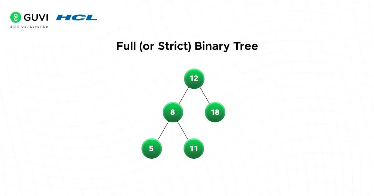
A full binary tree is one where every internal node has either two children or none. In other words, you’ll never see a node with just one child.
Why does this matter? Because full trees often appear in recursive structures like expression trees, where each operator acts on exactly two operands. It’s surprisingly common in parsing and evaluating formulas.
2. Perfect Binary Tree
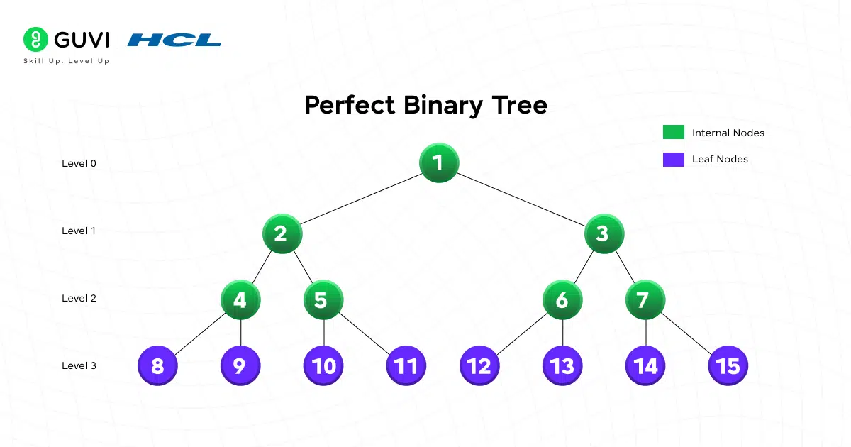
A perfect binary tree goes one step further: every internal node has two children and all leaves are on the same level. It’s the most symmetrical version possible. If the height is h, it has exactly 2^(h+1) – 1 nodes.
3. Complete Binary Tree
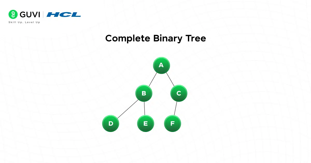
A complete binary tree is almost perfect; every level is filled except the last, and nodes on the last level are as far left as possible. This structure is extremely useful because it maps naturally to arrays (e.g. heaps), making it memory-efficient and cache-friendly.
4. Skewed (Degenerate) Binary Tree
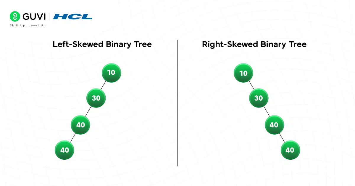
Imagine inserting sorted values into a BST without balancing: 1, 2, 3, 4, 5… You end up with a “linked list pretending to be a tree.” That’s a skewed tree; every node has only one child. Why should you care? Because this is the worst-case performance scenario, where operations degrade from O(log n) to O(n). Skewed trees are a warning sign that your tree might need balancing.
5. Balanced Binary Tree
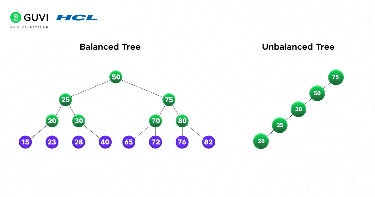
A balanced tree ensures that the height difference between the left and right subtrees of any node stays small (often ≤ 1). Height matters because tree height drives time complexity. If the tree stays roughly even, operations remain fast.
Most “real-world” tree structures (like AVL or Red-Black Trees) enforce balance automatically, but even if you don’t implement them, understanding the need for balance is key.
6. Binary Search Tree (BST)
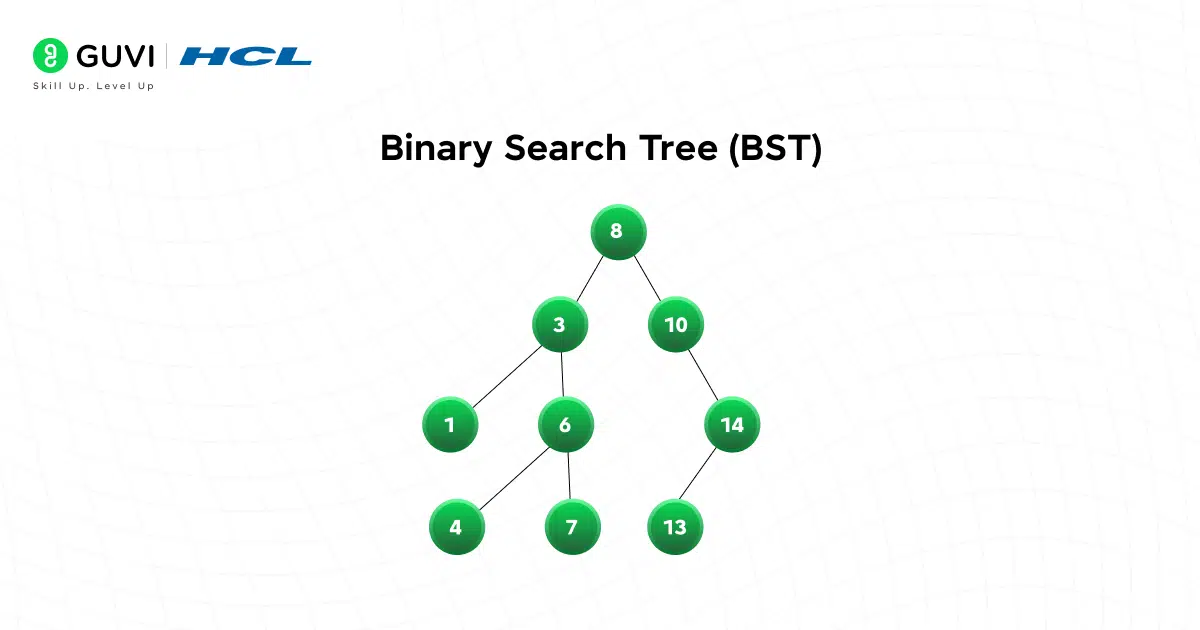
A BST adds ordering to the mix:
- Left subtree → smaller values
- Right subtree → larger values
This single rule makes BSTs powerful for search, insert, and delete operations. But BSTs only work well if they stay balanced. Otherwise, they become skewed and lose their advantage.
7. Heap (Min or Max)
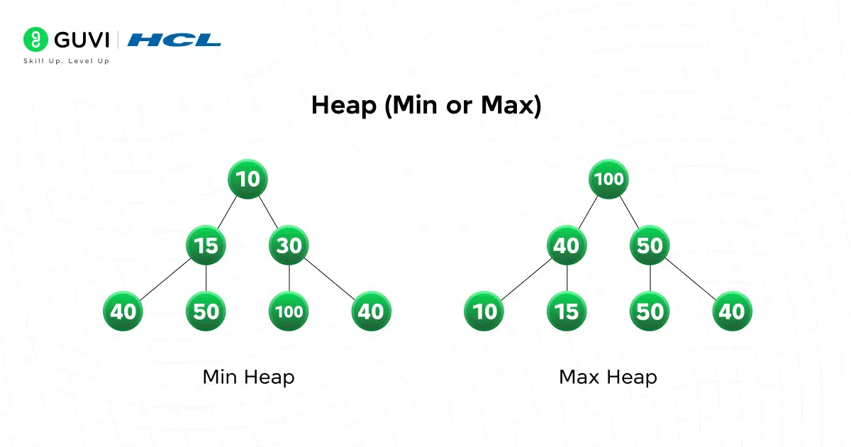
A heap is also a binary tree, but it has a different priority: parent-child ordering, not left-right ordering. In a min-heap, every parent is smaller than its children. Combined with the complete structure, heaps allow fast access to the min or max element, perfect for priority queues.
8. Expression Tree
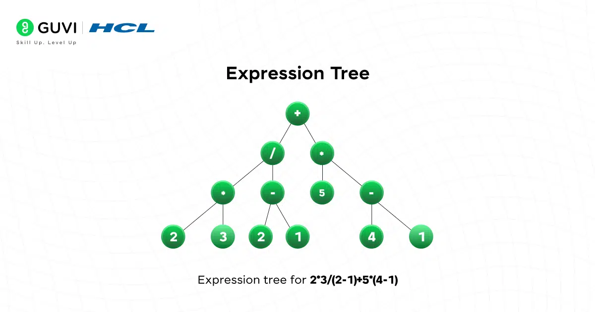
Expression trees represent mathematical expressions where:
- Leaves = operands (numbers/variables)
- Internal nodes = operators (+, *, etc.)
These trees are the backbone of compilers and calculators. They show how binary trees can represent structured logic, not just numbers.
If you want to read more about how binary trees in DSA pave the way for effective coding and its use cases, consider reading HCL GUVI’s Free Ebook: The Complete Data Structures and Algorithms Handbook, which covers the key concepts of Data Structures and Algorithms, including essential concepts, problem-solving techniques, and real MNC questions
Core Operations & Algorithms
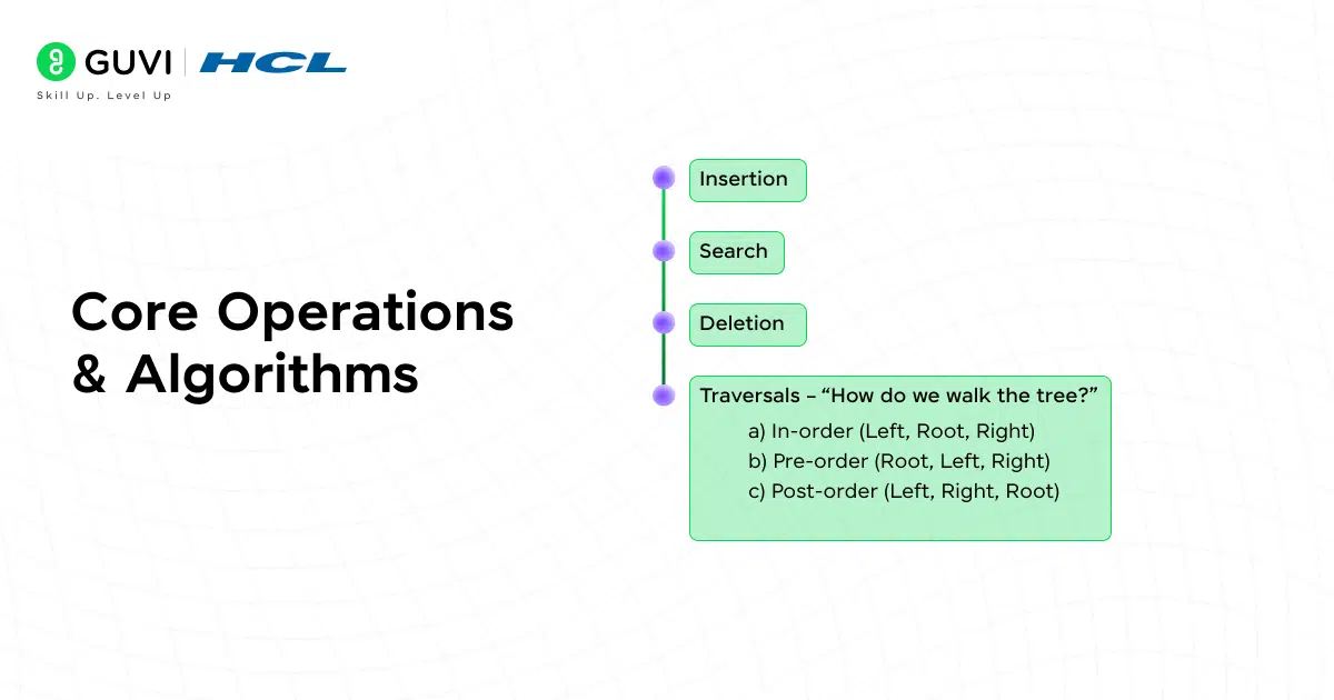
Now that you know the shapes of binary trees, let’s talk about what you can actually do with binary trees. Working with trees is all about performing operations like insert, search, delete, and traversal.
To keep things focused and practical, we’ll implement these on a Binary Search Tree (BST), since it’s the most common variant you’ll write manually.
We’ll start with the basic node in C++.
#include <bits/stdc++.h>

using namespace std;

struct Node {

    int key;

    Node* left;

    Node* right;

    Node(int k) : key(k), left(nullptr), right(nullptr) {}

};
1. Insertion
Inserting into a BST follows a simple idea: smaller values go left, larger values go right. We recurse until we find a null spot.
Node* insertBST(Node* root, int key) {

    if (!root) return new Node(key);

    if (key < root->key) {

        root->left = insertBST(root->left, key);

    } else if (key > root->key) {

        root->right = insertBST(root->right, key);

    }

    return root;

}
This keeps the BST property intact, but remember: if the tree becomes skewed, insertion becomes slow.
2. Search
BST search works the same way you’d search in a dictionary, narrowing the range step by step.
Node* searchBST(Node* root, int key) {

    if (!root || root->key == key) return root;

    if (key < root->key) return searchBST(root->left, key);

    return searchBST(root->right);

}
Average case: O(log n)
Worst case (skewed): O(n)
3. Deletion
Deletion is the trickiest BST operation because we have to rearrange nodes while keeping the order rule intact. There are three cases:
- Node has no children → just delete it.
- Node has one child → replace node with child.
- Node has two children → replace with in-order successor (smallest in right subtree), then delete that successor.
Node* findMin(Node* root) {

    while (root->left) root = root->left;

    return root;

}

Node* deleteBST(Node* root, int key) {

    if (!root) return nullptr;

    if (key < root->key) {

        root->left = deleteBST(root->left, key);

    } else if (key > root->key) {

        root->right = deleteBST(root->right, key);

    } else {

        if (!root->left && !root->right) {

            delete root;

            return nullptr;

        }

        if (!root->left || !root->right) {

            Node* child = root->left ? root->left : root->right;

            delete root;

            return child;

        }

        Node* succ = findMin(root->right);

        root->key = succ->key;

        root->right = deleteBST(root->right, succ->key);

    }

    return root;

}
4. Traversals – “How do we walk the tree?”
Traversal means visiting every node in a specific order. Each order gives you something different.
a) In-order (Left, Root, Right)
Returns sorted values in BST.

void inorder(Node* root) {

    if (!root) return;

    inorder(root->left);

    cout << root->key << " ";

    inorder(root->right);

}
b) Pre-order (Root, Left, Right)
Useful for copying or serializing.
void preorder(Node* root) {

    if (!root) return;

    cout << root->key << " ";

    preorder(root->left);

    preorder(root->right);

}
c) Post-order (Left, Right, Root)
Common for deleting the entire tree.
void postorder(Node* root) {

    if (!root) return;

    postorder(root->left);

    postorder(root->right);

    cout << root->key << " ";

}
d) Level-order (Breadth-first)
Visits one level at a time using a queue.
void levelOrder(Node* root) {

    if (!root) return;

    queue<Node*> q;

    q.push(root);

    while (!q.empty()) {

        Node* cur = q.front(); q.pop();

        cout << cur->key << " ";

        if (cur->left) q.push(cur->left);

        if (cur->right) q.push(cur->right);

    }

}
5. Height & Balance Check
Height = longest path from root to a leaf.
int height(Node* root) {

    if (!root) return -1;

    return 1 + max(height(root->left), height(root->right));

}
Balanced trees keep this height small. We can check the balance (difference ≤ 1) like this:
pair<int,bool> heightAndBalanced(Node* root) {

    if (!root) return {-1, true};

    auto [hl, bl] = heightAndBalanced(root->left);

    auto [hr, br] = heightAndBalanced(root->right);

    int h = 1 + max(hl, hr);

    bool balanced = bl && br && abs(hl - hr) <= 1;

    return {h, balanced};

}

bool isBalanced(Node* root) {

    return heightAndBalanced(root).second;

}
Once you understand why different tree shapes exist and how operations work under the hood, you’ll start recognizing trees everywhere: in compilers, search engines, databases, file systems, priority queues, and even AI models.
Use Cases & Applications
Binary trees show up everywhere once you start looking. Different problems lean on different guarantees: ordering, completeness, or shape.
1. Ordered data structures
BSTs (and their balanced cousins) back maps and sets when you need key order and predictable performance. You’ll see them underneath many standard library containers. Sorted iteration, range queries, and nearest-neighbor operations fall out naturally from in-order traversal.
2. Priority queues and scheduling
Heaps use the complete-tree shape to live happily inside arrays. They support fast insert and pop of the min/max element, so they’re staples in schedulers, simulation engines, and algorithms like Dijkstra’s. You’re not searching arbitrarily inside a heap; you’re repeatedly pulling the top priority.
3. Compilers and interpreters
Expression trees and ASTs model the structure of code and formulas. Traversal order becomes meaningful: pre-order for prefix notation, post-order for evaluation, in-order for pretty-printing. If you’ve ever walked an AST to apply transformations or analyses, you’ve driven a tree.
4. Compression and networking
Huffman coding builds an optimal prefix code using a binary tree where frequent symbols live closer to the root. Encoding is just following the left/right edges; decoding is walking until you hit a leaf. Fast, elegant, and a perfect marriage of shape and purpose.
5. Decision-making and games
Decision trees model branching choices. In games, search trees (like minimax with alpha–beta pruning) explore possible moves. Trees give you a clean way to represent alternate futures and prune bad paths early.
If you remember only one thing here, make it this: pick the tree whose invariants match your problem, order when you need sorted access, completeness for heap-like priorities, structure when representing syntax.
Implementation Tips & Pitfalls
The difference between a neat demo and production-grade code is in the edges: duplicates, nulls, memory, and testing. Here’s how to stay out of trouble.
- Decide your duplicate policy early: BSTs need a rule: reject duplicates, always send equals left or right, or store a count in the node. Pick one and stick to it.
- Guard against skew and deep recursion: Recursive insert/search is readable, but a skewed tree can push recursion depth high enough to risk a stack overflow. Keep iterative alternatives handy for traversals and consider randomized inserts (or a balanced structure) for adversarial input.
- Validate the BST property properly: Don’t just check immediate children. Use min/max bounds as you recurse, so every node is constrained by the entire path above it.
- Be deliberate about memory: Manual new and delete can leak memory if you exit early on errors or forget clean up. Prefer smart pointers (unique_ptr) if you’re building something serious.
- Keep I/O and structure separate: It’s tempting to print inside traversal functions. Better: pass a callback or collect results and print at the edge. This makes your traversals reusable for counting, mapping, or building new structures without coupling them to cout.
- Know when not to write your own: If your goal is reliable, general-purpose maps/sets, lean on well-tested library containers. Hand-rolled trees are great for learning or specialized needs, but maintenance and edge cases add up quickly.
Binary trees hide some surprisingly elegant math. For example, in every non-empty binary tree, the number of leaf nodes is always one more than the number of nodes with two children, a relationship that holds no matter how the tree is shaped. Even cooler? The number of different binary tree shapes you can form with n nodes is given by the Catalan numbers, a famous sequence that appears in everything from parsing expressions to counting valid parentheses. In other words, binary trees are not just practical, they’re deeply mathematical.
If you’re serious about mastering DSA in software development and want to apply it in real-world scenarios, don’t miss the chance to enroll in HCL GUVI’s IITM Pravartak and MongoDB Certified Online AI Software Development Course. Endorsed with NSDC certification, this course adds a globally recognized credential to your resume, a powerful edge that sets you apart in the competitive job market.
Conclusion
In conclusion, binary trees aren’t just another concept to memorize; they’re a way of thinking about data. Once you see how structure, ordering, and balance affect performance, you start recognizing why different tree types exist and when each one shines. A BST helps you search intelligently.
A heap helps you prioritize. Expression trees model logic. Self-balancing trees guarantee speed even in the worst case. And with just a few core operations: insert, search, delete, traverse, you can build incredibly powerful systems.
The more you work with binary trees, the more they stop feeling abstract and start feeling like tools you can shape to fit any problem. Master the patterns, respect the pitfalls, and binary trees will become one of the most versatile skills in your toolkit.
FAQs
1. What is the difference between a Binary Tree and a Binary Search Tree?
A binary tree is any tree where each node has up to two children. A BST adds ordering: left subtree < node < right subtree, which enables faster search and insert.
2. Why do we use binary trees in data structures?
Binary trees help organize data hierarchically, enabling efficient search, traversal, expression parsing, priority handling, and more. They’re also the foundation for advanced structures like heaps, BSTs, and segment trees.
3. What are the types of binary trees?
Common types include full, perfect, complete, skewed, balanced, binary search trees, heaps, and expression trees. Each type has its own structural rule and use case.
4. What are common operations on a BST?
The core operations are insertion, search, deletion, and traversal (in-order, pre-order, post-order, level-order). In a balanced BST, these run in O(log n) time.
5. What happens if a BST becomes unbalanced?
The tree can become skewed, increasing its height and causing performance to drop to O(n) for operations. To prevent this, self-balancing trees like AVL or Red-Black trees are used.


Did you enjoy this article?