
Linear Regression Model in Machine Learning: A Comprehensive Guide
Sep 04, 2025 6 Min Read 2839 Views
(Last Updated)
Have you ever wondered how Netflix always seems to know exactly what you’ll want to watch next, or how real estate websites manage to estimate house prices with such uncanny accuracy? One of the simplest yet most powerful tools in the machine learning toolbox, linear regression is often behind these digital predictions. Let’s break down how the linear regression model in machine learning works:
Table of contents
- What is a Linear Regression Model in Machine Learning?
- Types of Linear Regression
- Top Use Cases of Simple Linear Regression
- Top Use Cases of Multiple Linear Regression
- Simple Linear Regression and Multiple Linear Regression Key Differences Explained
- What is Supervised Regression?
- Why Choose Linear Regression for Supervised Regression Tasks?
- Drawbacks of the Linear Regression Model in Continuous Prediction
- Regression Analysis Tutorial: Step-by-Step Guide to Building a Linear Regression Model
- Step 1: Define the Supervised Regression Problem and Gather Data
- Step 2: Data Preparation for Linear Regression Model
- Step 3: Build and Train Your Linear Regression Model
- Step 4: Evaluate the Model Using Regression Coefficient Analysis
- Step 5: Interpret and Validate Linear Regression Model Results
- Step 6: Deploy and Maintain the Linear Regression Model
- Least Squares: The Mathematical Foundation of Linear Regression Model Training
- The Closed-Form Solution
- Why Least Squares Are So Powerful?
- Regression Coefficient and Mean Squared Error: Interpreting Model Outputs
- Regression Coefficient: Measuring Feature Impact
- Mean Squared Error: Assessing Prediction Quality
- Advanced Linear Regression Model Techniques
- Key Assumptions of Linear Regression
- Real-World Applications of Linear Regression Model in Supervised Regression
- The Future of Linear Regression Model in Machine Learning
- Conclusion
- FAQs
What is a Linear Regression Model in Machine Learning?

A linear regression model is a fundamental and powerful technique for supervised regression tasks in machine learning. Its goal is to model the relationship between one or more input variables (features) and a continuous output (target) variable.
Types of Linear Regression
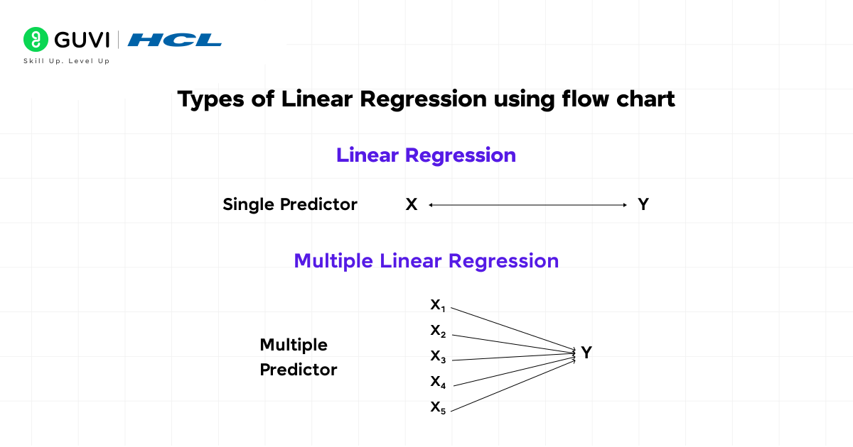
- Simple Linear Regression
Simple linear regression models the relationship between a single independent variable and a dependent variable through a straight line. It uses two parameters, slope and intercept to predict outcomes directly from one feature. This approach works well when one predictor drives the majority of variability in the response and when other variables exert negligible influence.
The mathematical form for simple linear regression (one input feature) is:
y = θ₀ + θ₁x
Where:
- y = predicted (target) value (continuous prediction)
- x = single input feature
- θ₀ = intercept of the best-fit line
- θ₁ = regression coefficient (slope)
Top Use Cases of Simple Linear Regression
- Estimating sales volume based on advertising expenditure.
- Predicting height from age in pediatric growth studies.
- Modeling temperature change over time in climate analysis.
- Forecasting weight from caloric intake in nutritional research.
Also Read: Must-Know Data Science Algorithms for Machine Learning
- Multiple Linear Regression
Multiple linear regression extends simple regression to include two or more independent variables. Additional predictors often improve accuracy when they each contribute unique information. However, complexity rises as the number of parameters grows.
Multiple linear regression extends this to include multiple predictors:
y = θ₀ + θ₁x₁ + θ₂x₂ + ⋯ + θₙxₙ
Where:
- x₁, x₂, …, xₙ are the input features (predictors)
- θ₁, θ₂, …, θₙ are their corresponding regression coefficients (each θᵢ quantifies the impact of feature xᵢ on the prediction)
- θ₀ remains the intercept
Top Use Cases of Multiple Linear Regression
- Housing market analysis incorporating square footage and location quality.
- Medical risk assessment using age and blood pressure, and cholesterol levels.
- Financial forecasting combines interest rates and GDP growth.
- Customer satisfaction modeling across price and service spee,d and product quality.
In summary:
Each regression coefficient (θᵢ) measures the expected change in the target value (y) for a one-unit increase in the corresponding feature (xᵢ). It holds all other features constant (in the case of multiple regression).
Take your skills to the next level! Join the AI & Machine Learning Course (with Intel Certification) to master linear regression, model evaluation, and advanced prediction techniques through hands-on projects. Enroll now to earn a globally recognized Intel certificate and accelerate your journey in data science!
Simple Linear Regression and Multiple Linear Regression Key Differences Explained
| Aspect | Simple Linear Regression | Multiple Linear Regression |
| Equation | y = θ₀ + θ₁·x₁ | y = θ₀ + θ₁·x₁ + θ₂·x₂ + … |
| Number of Predictors | one | two or more |
| Computational Complexity | low | Individual effects require care when features correlate |
| Interpretability | larger sample is needed to estimate multiple coefficients accurately | direct influence of a single feature |
| Multicollinearity Risk | none | high |
| Data Requirement | smaller dataset acceptable | amplifies as more features join the model |
| Sensitivity to Outliers | moderate | Forecasting house prices using area and location qualit,y and age of home |
| Use Case Example | predicting height from age | Predicting height from age |
What is Supervised Regression?
Supervised regression is a branch of supervised learning in machine learning. In this, the ultimate goal is to model the relationship between input variables or features and a continuous output variable or target. The algorithm is trained using labeled data or datasets in which both the input variables and their corresponding output values are known.
Common algorithms for supervised regression include:
- Linear regression
- Decision trees
- Random forest regression
- Support vector regression.
Why Choose Linear Regression for Supervised Regression Tasks?
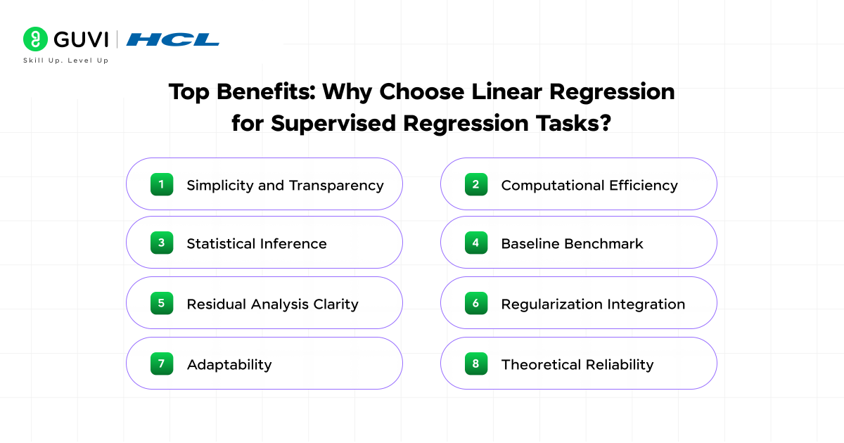
Data scientists and analysts rely on the linear regression model for a wide range of supervised regression problems because of its unique benefits:
- Simplicity and Transparency
The linear regression model is simple to grasp and clarify, mainly when dealing with straightforward linear regression. Every regression coefficient indicates what influence each feature has on the final result.
- Computational Efficiency
The least squares method allows for the estimation of coefficients in a linear regression model. This can be done even with large datasets, and it can be done quite efficiently.
- Statistical Inference
One can evaluate the statistical significance of each regression coefficient through hypothesis testing. This makes the model useful not just for making predictions but also for doing inferential analysis.
- Baseline Benchmark
A model of linear regression will often act as the entry point in any given regression analysis tutorial. At this point, the user will have been shown how to set up a model and get results for something that is relatively simple in the world of regression. From here, we will try to move to more complex scenarios and see how they perform relative to our simple baseline.
- Residual Analysis Clarity
The quality of data and the limitations of a model can be easily identified by looking at the differences (residuals) between the actual and predicted values.
- Regularization Integration
Ridge regression and Lasso regression are extensions of regularized regression that use regularization to not only prevent overfitting but also to select important features, those that really have an effect on the dependent variable from a set of possible features.
- Adaptability
Real-time (online) and batch learning scenarios are both served well by linear regression models, which makes these models quite adaptable.
- Theoretical Reliability
The assumptions and underlying mathematics of linear regression have been extensively studied and validated. It further fosters a high level of trust in the method among practitioners.
Drawbacks of the Linear Regression Model in Continuous Prediction
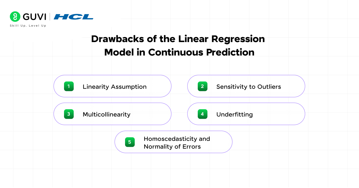
The linear regression model is not always the best tool for every continuous prediction task, despite its strengths. Here are the key challenges:
- Linearity Assumption
The relationship between the predictors and the target must be linear for both simple and multiple linear regression to yield satisfactory results. The model’s predictive confidence is enormously reduced if your data contains non-linear relationships.
- Sensitivity to Outliers
Outliers can disproportionately influence the fitted line and distort regression coefficients, which further leads to misleading results.
- Multicollinearity
The reliability of the regression coefficients decreases as their variance increases when predictors in multiple linear regression are highly correlated. It further makes interpretation and inference more difficult.
- Underfitting
The predictive power of a linear regression model is greatly limited when applied to data with complex or nonlinear patterns. In real-world scenarios, the assumption that all predictor variables have a purely linear influence is often violated, which can result in poor predictive performance.
- Homoscedasticity and Normality of Errors
Violations of the assumptions that errors are equally (homoscedastic) and normally distributed can negatively impact the validity of statistical inference and the overall reliability of the model.
Regression Analysis Tutorial: Step-by-Step Guide to Building a Linear Regression Model
Let’s walk through a regression analysis tutorial for applying the linear regression model in practice:
Step 1: Define the Supervised Regression Problem and Gather Data
Start by clearly defining your supervised regression goal. For example, predicting house prices using features such as square footage, number of bedrooms, location, and age of property. Collect a dataset that includes both the target variable (e.g., price) and relevant predictors.
Step 2: Data Preparation for Linear Regression Model
- Handle Missing Data: Impute missing values using mean or a suitable method.
- Standardize or Normalize Features: Especially important in multiple linear regression for comparability.
- Encode Categorical Variables: Use one-hot encoding or ordinal encoding as needed.
- Split Data: Divide your data into training and testing sets (commonly 80% train, 20% test) for model validation.
Step 3: Build and Train Your Linear Regression Model
- Import the Model: Use LinearRegression from scikit-learn or a similar package.
- Fit the Model: Apply the least squares method to estimate the regression coefficients.
- Objective Function: The model minimizes the mean squared error (MSE).
Learn More: 10 Best AI and ML Courses For You [Free + Paid]
Step 4: Evaluate the Model Using Regression Coefficient Analysis
- Analyze Coefficients: Examine the sign and magnitude of each regression coefficient. Is the direction of influence as expected?
- Performance Metrics: Evaluate mean squared error and R² (coefficient of determination) on your test data.
- Residual Analysis: Plot and inspect residuals for patterns or trends missed by the model.
Step 5: Interpret and Validate Linear Regression Model Results
Each regression coefficient represents the change in the target variable for a one-unit increase in the corresponding feature, holding all others constant (important in multiple linear regression). In multiple regression, always check for multicollinearity (using variance inflation factors, VIF).
Step 6: Deploy and Maintain the Linear Regression Model
Once validated, serialize your linear regression model (e.g., using pickle or joblib in Python). Deploy it via an API (like Flask or FastAPI) so it can make predictions on new data. Continuously monitor prediction performance and retrain with new data. Also, log both actual and predicted values for ongoing improvement.
Least Squares: The Mathematical Foundation of Linear Regression Model Training
The least squares method serves as the core algorithm behind both simple linear regression and multiple linear regression. This approach determines the optimal set of regression coefficients by minimizing the sum of squared differences, called residuals, between the actual observed values and those predicted by the model.
The Closed-Form Solution
In matrix notation for multiple linear regression, the optimal coefficient vector is calculated as:
θ = (XᵀX)^(-1)Xᵀy
- XX: Feature matrix representing input variables
- yy: Target vector containing observed outputs
Why Least Squares Are So Powerful?
This method not only provides the most accurate linear fit under the model’s assumptions, but also ensures that the resulting estimates are unbiased and have the smallest possible variance among all linear unbiased estimators (thanks to the Gauss-Markov theorem).
Regression Coefficient and Mean Squared Error: Interpreting Model Outputs
Understanding and evaluating a linear regression model requires more than just fitting a line; it hinges on interpreting the model’s key metrics.
Regression Coefficient: Measuring Feature Impact
A regression coefficient quantifies the effect of each input variable on the output, indicating not just direction (positive/negative) but also magnitude. In multiple linear regression, it represents the unique contribution of a predictor, adjusted for all others.
Mean Squared Error: Assessing Prediction Quality
MSE = (1/n) Σ (yi – ŷi)²
The mean squared error (MSE) captures the average squared difference between observed and predicted values. It is widely used as the primary metric for continuous prediction tasks because it penalizes large errors more strongly, therefore ensuring that models not simply fit but generalize well.
Advanced Linear Regression Model Techniques
Moving beyond basic fitting, modern practitioners leverage advanced strategies to level up multiple linear regression and prevent pitfalls.
Key Assumptions of Linear Regression
The successful application of linear regression depends on the following assumptions:
- Linearity: The relationship between predictors and the target must be straight-line (linear and additive).
- Normality of Errors: Residuals (prediction errors) should follow a normal distribution to ensure valid inference.
- Homoscedasticity: The spread of residuals must remain constant for all values of the predictors.
- No Multicollinearity: Input features in multiple linear regression should not be highly correlated. High multicollinearity leads to unstable coefficient estimates.
- Independence: Residuals should be uncorrelated, especially important for time series data to avoid misleading trends due to autocorrelation.
Real-World Applications of Linear Regression Model in Supervised Regression
Linear regression models are the backbone of modern analytics across industries. Here are just a few examples where continuous prediction powered by supervised regression drives value:
- Healthcare: Estimating patient risk scores using age and history (multiple linear regression).
- Finance: Predicting credit risk or stock market returns from economic indicators.
- Real Estate: Calculating house prices using square footage and neighborhood features.
- Energy: Forecasting power consumption based on weather and time of day.
- Marketing: Estimating customer lifetime value or campaign effectiveness from engagement metrics.
- Agriculture: Predicting crop yield using climate data and soil properties (multiple linear regression).
- Transport: Modeling demand for ride-sharing or logistics operations from time and event data.
The Future of Linear Regression Model in Machine Learning
While more sophisticated algorithms like tree ensembles and neural networks are rising in popularity, the linear regression model endures because it is interpretable and mathematically robust. Every regression analysis tutorial, whether for a classroom or a professional setting begins here for a reason.
Modern advancements like online learning (adapting to new data streams in real-time), feature selection with Lasso, and integration into pipelines with other machine learning models keep linear regression relevant and evolving.
Conclusion
The linear regression model stands as the cornerstone of supervised regression and the starting point in every credible regression analysis tutorial. Thus, no matter if you are exploring simple linear regression for quick insights or using multiple linear regression for multi-factor forecasting, understanding the principles of least squares and model assumptions will make you a stronger and more reliable data scientist.
FAQs
Q1: What types of data are best suited for linear regression models?
Linear regression is best for numerical data where relationships between variables are expected to be approximately linear. Categorical variables should be encoded before use.
Q2: How is linear regression different from logistic regression?
Linear regression predicts continuous numeric outcomes. On the other hand, logistic regression predicts probabilities for binary or categorical outcomes.
Q3: Can linear regression handle missing values automatically?
No, missing values must be handled before modeling, typically by imputation or removing incomplete records.
Q4: Is it possible to use linear regression for time series forecasting?
Yes, linear regression can be used with time series. Although, it requires careful handling of temporal structure and checks for autocorrelation.
Q5: What does it mean if the R-squared value is close to zero?
It suggests that the linear regression model explains very little of the variance in the target variable and may not be suitable for the dataset.
Q6: Why is feature scaling sometimes important for linear regression?
Scaling guarantees that all features contribute equally, especially when using regularization or when predictor values vary widely in magnitude.
Q7: Can linear regression be used for real-time predictions?
Yes, once trained, linear regression models are fast and efficient. This makes them suitable for real-time or streaming prediction tasks.
Q8: How do you check if your linear regression model is overfitting?
If the model performs well on training data but poorly on new (test) data, it is likely overfitting. Regularization or simpler models can help.








Did you enjoy this article?