Policy Gradient Methods in Reinforcement Learning

Policy gradient methods enable reinforcement learning agents to learn optimal behaviors by directly optimizing the policy rather than learning value functions.
These methods power advanced AI systems from robotics to game playing and language model alignment.
This guide explains how policy gradient methods work, key algorithms, and practical implementation considerations.

Direct Answer

Policy Gradient Methods are reinforcement learning algorithms that optimize the policy directly by computing gradients of expected return with respect to policy parameters. Instead of learning a value function and deriving a policy from it, policy gradient methods parameterize the policy (typically as a neural network) and use gradient ascent to maximize expected cumulative reward. Key algorithms include REINFORCE, Actor-Critic, PPO, and TRPO, which balance exploration, stability, and sample efficiency for different applications.

TL;DR Summary Box

• Policy gradient methods optimize the policy directly using gradient ascent.
• REINFORCE is the simplest but has high variance.
• Actor-Critic methods reduce variance by learning value functions.
• PPO and TRPO add constraints for stable, reliable training.
• These methods excel in continuous action spaces and complex environments.

What Are Policy Gradient Methods?

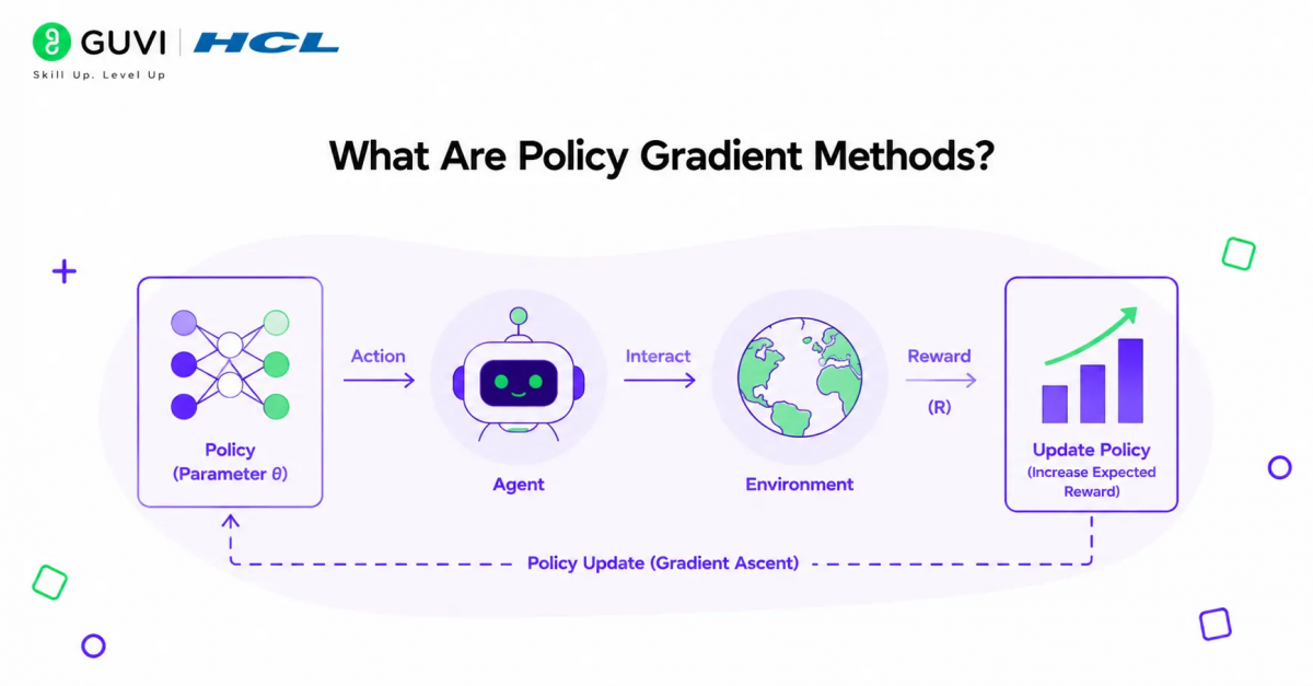
Policy gradient methods are a family of reinforcement learning algorithms that learn the policy directly, without relying on value functions to derive actions.

The Policy in RL

In reinforcement learning, a policy defines how an agent behaves:

• Policy (π): A function that maps states to actions
• Deterministic policy: π(s) = a (always takes same action in state s)
• Stochastic policy: π(a|s) = probability of taking action a in state s

Policy gradient methods parameterize the policy with parameters θ (typically neural network weights) and optimize these parameters to maximize expected return.

Why Policy Gradients?

Policy gradient methods offer several advantages over value-based methods (like Q-learning):

Advantages:

• Continuous action spaces: Natural handling of continuous actions (robotics, control)
• Stochastic policies: Can learn optimal stochastic behaviors
• Simplicity: Often simpler to implement than value-based methods
• Convergence: Better convergence properties in some domains
• High-dimensional actions: Scale better to high-dimensional action spaces

Disadvantages:

• Sample inefficiency: Often require more samples than value-based methods
• Local optima: Can converge to local rather than global optima
• High variance: Gradient estimates can have high variance
• Hyperparameter sensitivity: Sensitive to learning rate and other hyperparameters

Policy gradient methods directly optimize the policy by sampling actions and updating parameters in the direction that increases expected return, enabling RL in high-dimensional or continuous action spaces.Master AI & ML at HCL GUVI: Artificial Intelligence and Machine Learning. 

The Policy Gradient Theorem

The foundation of all policy gradient methods is the policy gradient theorem, which provides a way to compute gradients of expected return.

Objective Function

The goal is to maximize expected cumulative reward:

J(θ) = E[Σ γ^t * r_t]

Where:

• θ are the policy parameters
• γ is the discount factor (0 < γ ≤ 1)
• r_t is the reward at time t
• The expectation is over trajectories sampled from the policy

Policy Gradient Theorem

The theorem states that the gradient of the objective is:

∇J(θ) = E[∇log π(a|s; θ) * Q(s,a)]

This means:

• Compute the gradient of the log probability of taken actions
• Weight by the action-value (how good that action was)
• Take expectation over the trajectory distribution

Intuition

The policy gradient theorem provides an elegant update rule:

• If an action leads to high return: Increase its probability (positive gradient)
• If an action leads to low return: Decrease its probability (negative gradient)
• Magnitude: Proportional to how much better/worse the action was

This creates a natural learning signal that reinforces good actions and discourages bad ones.

How REINFORCE Works

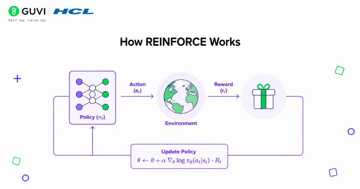
REINFORCE (Monte Carlo Policy Gradient) is the simplest policy gradient algorithm.

Algorithm:

1. Sample trajectory: Run policy to collect episode (s₁, a₁, r₁, …, s_T, a_T, r_T)
2. Compute returns: For each time step, calculate cumulative future reward
3. Compute gradients: ∇log π(a_t|s_t) * G_t for each step
4. Update policy: θ ← θ + α * ∇J(θ)

Return calculation:

G_t = r_t + γr_{t+1} + γ²r_{t+2} + ... + γ^{T-t}r_T

This is the total discounted reward from time t onward.

REINFORCE with Baseline

A critical improvement reduces variance by subtracting a baseline:

∇J(θ) = E[∇log π(a|s) * (Q(s,a) - b(s))]

Where b(s) is a baseline (typically a value function estimate).

Why this helps:

• Subtracting baseline doesn’t change expected gradient (unbiased)
• Reduces variance significantly
• Makes learning more stable and efficient
• Common baseline: learned value function V(s)

Advantages of REINFORCE

• Simple: Easy to understand and implement
• Model-free: Doesn’t require environment model
• Unbiased: Gradient estimate is unbiased
• General: Works in any environment

Limitations of REINFORCE

• High variance: Monte Carlo returns have high variance
• Sample inefficient: Requires many episodes to learn
• Slow learning: Updates only after complete episodes
• Unstable: Can be unstable without careful tuning

Actor-Critic Methods

Actor-Critic methods combine policy gradient with value function learning to reduce variance.

The Actor-Critic Architecture

Two components:

1. Actor: The policy π(a|s; θ) that selects actions
2. Critic: The value function V(s; w) that evaluates states

How it works:

• Actor proposes actions based on current policy
• Critic evaluates how good the resulting states are
• Use critic’s evaluation to update actor with lower variance
• Both actor and critic are updated simultaneously

Advantage Function

Actor-Critic methods use the advantage function instead of raw returns:

A(s,a) = Q(s,a) - V(s)

This measures how much better an action is compared to the average action in that state.

Benefits:

• Lower variance than using raw returns
• Centers the learning signal around zero
• Faster, more stable learning
• Better credit assignment

A2C (Advantage Actor-Critic)

A2C is a synchronous, on-policy actor-critic algorithm.

Key features:

• On-policy: Uses current policy for sampling
• Synchronous: Single agent or multiple parallel agents
• Advantage estimation: Uses n-step returns for advantage
• Simple: Relatively simple to implement

Update rules:

• Critic: Minimize TD error: L = (r + γV(s’) – V(s))²
• Actor: Maximize: ∇log π(a|s) * A(s,a)

A3C (Asynchronous Advantage Actor-Critic)

A3C extends A2C with asynchronous parallel agents.

Key innovations:

• Multiple agents: Multiple workers explore the environment in parallel
• Asynchronous updates: Workers update global parameters independently
• Faster learning: Parallel exploration speeds up training
• Better exploration: Different agents explore different parts of state space

Architecture:

• Global shared parameters (actor and critic)
• Multiple worker threads
• Each worker: collects gradients, updates global parameters
• No locking required (asynchronous updates)

Advanced Policy Gradient Methods – TRPO (Trust Region Policy Optimization)

TRPO adds constraints to ensure stable, monotonic policy improvement.

Key idea:

Instead of unconstrained gradient ascent, TRPO constrains the policy update to stay within a “trust region” where the approximation is accurate.

Constraint:

Limit the KL divergence between old and new policy:

KL(πold || π_new) ≤ δ

This ensures:

• Policy doesn’t change too dramatically
• Updates are in regions where approximation is valid
• More stable, reliable learning

Advantages:

• Stable: Guaranteed monotonic improvement (theoretically)
• Robust: Less sensitive to hyperparameters
• Sample efficient: Better than REINFORCE and basic actor-critic

Limitations:

• Complex: More complex implementation
• Computationally expensive: Requires second-order optimization
• Slow: Slower per iteration than simpler methods

PPO (Proximal Policy Optimization)

PPO simplifies TRPO while maintaining similar performance, becoming one of the most popular RL algorithms.

Key innovation:

Instead of hard constraints, PPO uses a clipped surrogate objective that penalizes large policy updates.

Clipped objective:

L^CLIP(θ) = E[min(r_t(θ) A_t, clip(r_t(θ), 1-ε, 1+ε) A_t)]

Where:

• r_t(θ) = π_new(a|s) / π_old(a|s) (probability ratio)
• ε is the clipping parameter (typically 0.1–0.3)
• A_t is the advantage estimate

How clipping works:

• If advantage is positive (good action):
  • Want to increase probability
  • But clip prevents increasing too much (> 1+ε)
• If advantage is negative (bad action):
  • Want to decrease probability
  • But clip prevents decreasing too much (< 1-ε)

Advantages of PPO:

• Simple: Much simpler to implement than TRPO
• Stable: Similar stability to TRPO
• Sample efficient: Good sample efficiency
• Fast: Faster per iteration than TRPO
• Robust: Works well across many domains

Applications:

• Game playing (Dota 2, etc.)
• Robotics control
• Language model alignment (early RLHF systems)
• Continuous control tasks

Policy gradient methods directly optimize the policy by sampling actions and updating parameters in the direction that increases expected return, enabling RL in high-dimensional or continuous action spaces.Master AI & ML at HCL GUVI: Artificial Intelligence and Machine Learning. 

Common Mistakes to Avoid

• Not using baseline: REINFORCE without baseline has extremely high variance
• Wrong learning rate: Most common cause of failure
• Ignoring advantage estimation: Using raw returns instead of advantages
• No entropy regularization: Policy collapses to deterministic too quickly
• Improper normalization: Not normalizing observations or advantages
• Overfitting to samples: Too many epochs on same data in PPO
• Poor exploration: Insufficient exploration leads to local optima
• Not monitoring KL divergence: In PPO, KL should stay in reasonable range
• Ignoring reward scaling: Large rewards can cause instability
• No early stopping: Train until performance degrades

What Should You Do Next?

Use this practical checklist:

1. Start with REINFORCE to understand fundamentals
2. Implement REINFORCE with baseline for variance reduction
3. Move to Actor-Critic (A2C) for better performance
4. Try PPO for state-of-the-art results
5. Tune hyperparameters carefully (learning rate is critical)
6. Use advantage estimation (GAE) for better credit assignment
7. Monitor training metrics (reward, KL divergence, entropy)
8. Implement proper normalization (observations, advantages)
9. Add entropy regularization for better exploration
10. Validate on benchmark environments (CartPole, Pendulum, etc.)

Conclusion

Policy Gradient Methods provide a powerful framework for reinforcement learning by directly optimizing the policy using gradient ascent. From the simple REINFORCE algorithm to sophisticated methods like PPO and TRPO, these techniques enable agents to learn complex behaviors in continuous action spaces and high-dimensional environments.

The key insight is that by computing gradients of expected return with respect to policy parameters, we can use gradient ascent to improve the policy iteratively. Actor-Critic methods reduce variance by learning value functions, while PPO and TRPO add constraints for stable, reliable training.

For practitioners, PPO offers the best balance of performance, stability, and implementation complexity, making it the default choice for most applications. However, understanding simpler methods like REINFORCE and Actor-Critic provides crucial intuition for debugging and improving policy gradient algorithms.

FAQs