Simulated Annealing Algorithm Explained

The simulated annealing algorithm is a probabilistic optimization technique used to find a good or near-optimal solution to difficult problems. It is especially useful when the search space is large and contains many possible solutions.

TL;DR: Summary

• Simulated annealing is a probabilistic optimization algorithm that finds near-optimal solutions by occasionally accepting worse solutions to escape local optima.
• The algorithm balances exploration and refinement using a temperature parameter that gradually decreases through a cooling schedule.
• Simulated Annealing is widely used in routing, scheduling, machine learning, chip design, and other complex optimization problems where exact solutions are difficult to find.

What Is the Simulated Annealing Algorithm?

Unlike simple optimization methods that always move toward an immediately better solution, the Simulated Annealing algorithm may sometimes accept a worse solution. This helps it escape local optima and explore more promising areas of the search space.

Simulated annealing is a probabilistic optimization method that escapes local minima to find near-global optima. Learn AI & ML with HCL GUVI’s Artificial Intelligence and Machine Learning course. 

How the Simulated Annealing Algorithm Works

The simulated annealing algorithm begins with an initial solution and an initial temperature. It then repeatedly creates nearby solutions and decides whether to accept them.

1. Selecting a Neighboring Solution

A neighboring solution is created by making a small change to the current solution. For example, in a route optimization problem, the algorithm may swap the positions of two cities.

The quality of this new solution is then compared with the quality of the current solution.

2. Accepting Better Solutions

If the new solution is better than the current solution, it is accepted immediately. In a minimization problem, this means the new solution has a lower cost.

Accepting better solutions allows the algorithm to move toward improved results.

3. Accepting Worse Solutions

If the new solution is worse, it may still be accepted with a certain probability. This probability depends on two factors:

• How much worse the new solution is.
• The current temperature.

The common acceptance formula is:

Here:

• PPP is the probability of accepting the worse solution.
• ΔE\Delta EΔE is the increase in cost or energy.
• TTT is the current temperature.
• eee is the mathematical constant approximately equal to 2.718.

At a high temperature, the algorithm is more willing to accept worse solutions. At a low temperature, it becomes more selective.

The Role of Temperature

Temperature controls the balance between exploration and exploitation in the Simulated Annealing algorithm.

1. High Temperature and Exploration

At the beginning, the temperature is usually high. The algorithm can accept many worse solutions, allowing it to explore different regions of the search space.

This prevents the algorithm from becoming trapped in a local optimum too early.

2. Low Temperature and Refinement

As the temperature decreases, the algorithm becomes less likely to accept worse solutions. It gradually focuses on improving the current solution.

This process helps the algorithm refine its result and move toward a stable solution.

Cooling Schedules in Simulated Annealing

A cooling schedule determines how the temperature decreases during execution. Choosing the right schedule is important because cooling too quickly may produce a poor solution, while cooling too slowly may increase execution time.

1. Exponential Cooling

Exponential cooling reduces the temperature by multiplying it by a constant factor:

Tnew=αTT_{\text{new}} = \alpha TTnew​=αT

Here, α\alphaα is usually a value between 0 and 1.

This is one of the most commonly used cooling methods because it is simple and practical.

2. Linear Cooling

Linear cooling decreases the temperature by a fixed amount after each iteration:

Tnew=T−cT_{\text{new}} = T – cTnew​=T−c

Here, ccc is a constant cooling value. This approach is easy to implement but may not work equally well for every problem.

3. Logarithmic Cooling

Logarithmic cooling reduces the temperature more slowly than many other methods. It can produce strong theoretical results, but it may require more iterations and therefore more processing time.

Simulated Annealing Algorithm Steps

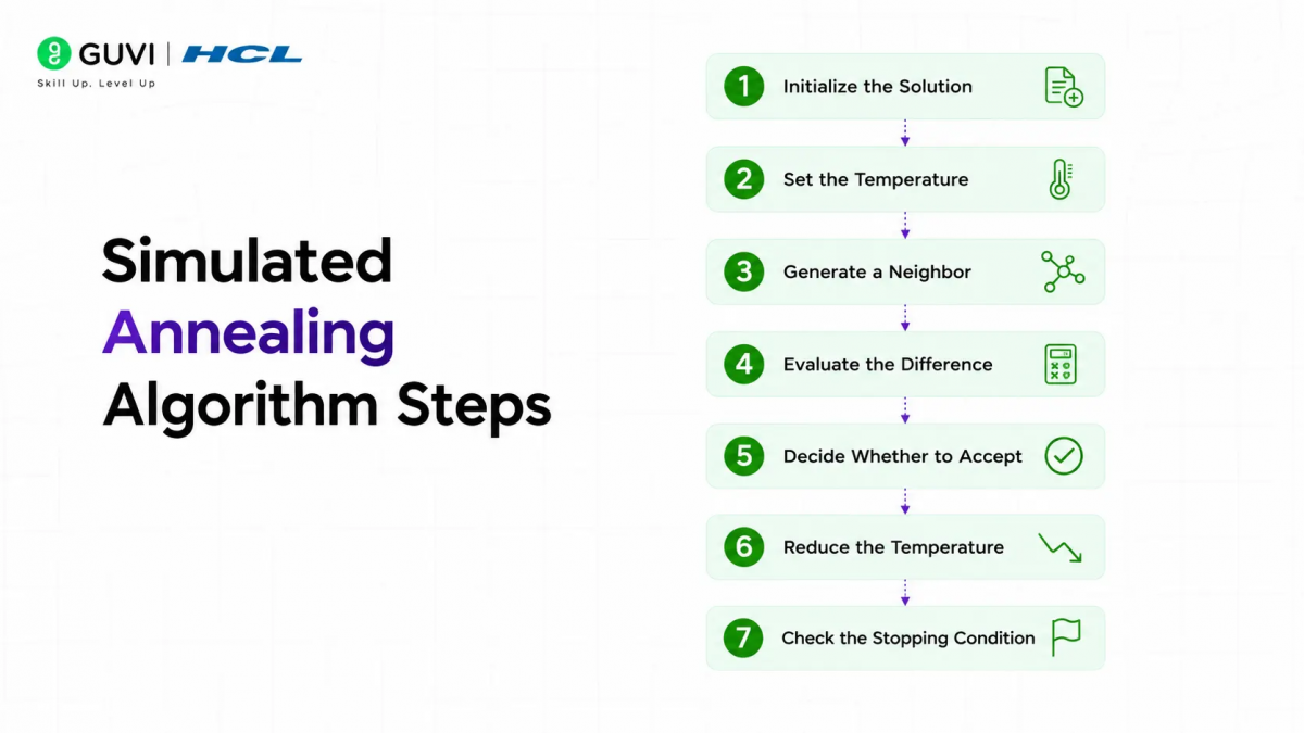
The general process can be summarized as follows:

Step 1: Initialize the Solution

Choose an initial solution, either randomly or using a simple starting strategy.

Step 2: Set the Temperature

Choose a high initial temperature that allows broad exploration.

Step 3: Generate a Neighbor

Create a new solution by making a small change to the current solution.

Step 4: Evaluate the Difference

Calculate the difference between the new solution and the current solution.

Step 5: Decide Whether to Accept

Accept the new solution if it is better. If it is worse, accept it according to the temperature-based probability.

Step 6: Reduce the Temperature

Apply the selected cooling schedule.

Step 7: Check the Stopping Condition

Continue until the temperature becomes very low, the maximum number of iterations is reached, or no meaningful improvement occurs.

To dive deeper into machine learning, explore our curated list of top AI/ML blogs 

Simulated Annealing Pseudocode

text

Choose an initial solution

Set the initial temperature

While the stopping condition is not reached:

    Generate a neighboring solution

    Calculate the change in cost

    If the new solution is better:

        Accept the new solution

    Else:

        Calculate the acceptance probability

        Accept the new solution based on that probability

    Reduce the temperature

Return the best solution found

Applications of Simulated Annealing

The simulated annealing algorithm is useful in many optimization problems.

1. Scheduling Problems

It can help assign employees, machines, or tasks to time slots while minimizing delays and conflicts.

2. Traveling Salesperson Problem

The algorithm can search for a short route that visits multiple locations exactly once before returning to the starting point.

3. Circuit and Chip Design

It can optimize the placement of components to reduce connection length, power consumption, or manufacturing complexity.

4. Machine Learning

Simulated Annealing can be used for feature selection, parameter optimization, and training problems where traditional methods may become trapped in poor solutions.

5. Resource Allocation

Businesses can use it to assign limited resources to projects while balancing cost, time, and performance.

Advantages of Simulated Annealing

• Its ability to accept worse solutions helps it move away from local optima and search for better global solutions.
• It can handle large and irregular search spaces where exact optimization may be impractical.
• The algorithm can be adapted to different problems by changing the neighborhood function, objective function, and cooling schedule.

Simulated annealing is a probabilistic optimization method that escapes local minima to find near-global optima. Learn AI & ML with HCL GUVI’s Artificial Intelligence and Machine Learning course. 

Limitations of Simulated Annealing

• Although the algorithm can find excellent solutions, it may not always return the global optimum within a practical amount of time.
• The initial temperature, cooling rate, number of iterations, and neighborhood design can strongly affect performance.
• A carefully tuned cooling schedule may require many iterations, especially for large and complex problems.

Best Practices for Using Simulated Annealing

1. Choose a Suitable Neighbor Function

The neighbor function should make meaningful but manageable changes. Very small changes may slow exploration, while very large changes may make the search unstable.

2. Start With a High Temperature

The initial temperature should be high enough to allow exploration. If it is too low, the algorithm may behave like basic hill climbing.

3. Cool Gradually

A gradual cooling schedule generally provides better exploration and refinement than a schedule that drops the temperature too quickly.

4. Keep the Best Solution

Always store the best solution found during the search. The final current solution may not be the best one encountered.

Conclusion

The simulated annealing algorithm is a flexible optimization method inspired by the controlled cooling of heated materials. It explores a solution space by accepting better solutions and occasionally accepting worse ones, especially during the early stages.

Its ability to escape local optima makes it useful for routing, scheduling, design, machine learning, and resource allocation. With a suitable temperature, cooling schedule, and neighborhood strategy, simulated annealing can produce high-quality solutions to problems that are difficult to solve using traditional methods.

FAQs