


The Normal Distribution and Z-Scores
The Normal Distribution and Z-Scores
The normal distribution is a symmetric, bell-shaped curve described by two numbers: the mean μ, which sets its center, and the standard deviation σ, which sets its width.
Many measurements, such as heights and test scores, approximate this shape, and many statistical methods assume it.
The 68-95-99.7 Rule
- About 68% of values fall within 1σ of the mean.
- About 95% fall within 2σ.
- About 99.7% fall within 3σ.
Z-Score
z = (x − μ) / σ
- z: the number of standard deviations a value sits above or below the mean. A negative z means below the mean.
- x: the value being checked.
- μ: the mean of the distribution.
- σ: the standard deviation of the distribution.
Converting values to z-scores puts them on a common scale, allowing you to compare scores measured in different units. Values with a z-score beyond about ±3 are often flagged as outliers.
Example: Exam scores are normal with mean 70 and standard deviation 10. Find the z-score for a mark of 85, the share of students scoring below 85, and the share scoring between 60 and 80.
- z = (85 − 70) / 10 = 1.5
- From the standard normal table, P(Z < 1.5) ≈ 0.9332, so about 93.3% score below 85.
- Marks of 60 and 80 correspond to z = −1 and z = +1, so the share between them is about 68.3%.
from scipy.stats import norm

print(norm.cdf(1.5))
print(norm.cdf(1) - norm.cdf(-1))
Code Explanation:
- norm.cdf(1.5) returns the probability that a standard normal value is below 1.5, which is about 0.9332.
- norm.cdf(1) - norm.cdf(-1) subtracts the area below −1 from the area below +1, leaving the area between them, about 0.6827.
- The same idea is used when features are standardized before modelling: each value is replaced by its z-score.
Probability and Statistics for Data Science
AP
Abhishek Pati

Recommended Handbooks

C++ Handbook
Level up your programming skills with our C++ Tutorials hub, guiding you from beginner to advanced. Start your journey now!

Python Basics Handbook
Level up your programming skills with our Python Tutorials hub, guiding you from beginner to advanced. Start your journey now!

Javascript Handbook
Level up your programming skills with our JavaScript Tutorials hub, guiding you from beginner to advanced. Start your journey now!
Building a Random Joke Generator Using ReactJS
Build a React app that fetches and displays random programming jokes using JokeAPI. Simple, fun, and perfect for beginners learning API calls and state management.
Build a Character Counter in React JS
Start your first project in React JS by building an interactive character counter application.
Build Your QR Code Generator using React JS
Start your first project in React JS by building a dynamic QR generator application.
Build a Birthday Reminder App using React JS
Start your first project in React JS by building a dynamic Birthday Reminder app that uses components and state to manage and display a list of birthdays.

Building BMI Calculator Using ReactJS
Build a responsive BMI Calculator using React that calculates BMI based on user input and displays the health status. Learn components, hooks, styling, and deploy it live on Netlify.
Building Random Password Generator using ReactJS
A React-based app to generate strong, customizable passwords with copy-to-clipboard support. Live and responsive via Netlify.
Temperature Converter Project in React
A beginner-friendly React app that converts temperatures between Celsius, Fahrenheit, and Kelvin with real-time results and clean CSS styling. Live on Netlify.
Building a To-Do List App Using ReactJS
Build a React To-Do List App that lets users add, edit, complete, and delete tasks in real-time. Clean UI, no backend, and perfect for mastering React basics.
Building a Weather App Project Using ReactJS
Build a React app that fetches and displays real-time weather data with animated icons, live clock, and a sleek UI. Great for beginners to learn React, APIs, and state management.
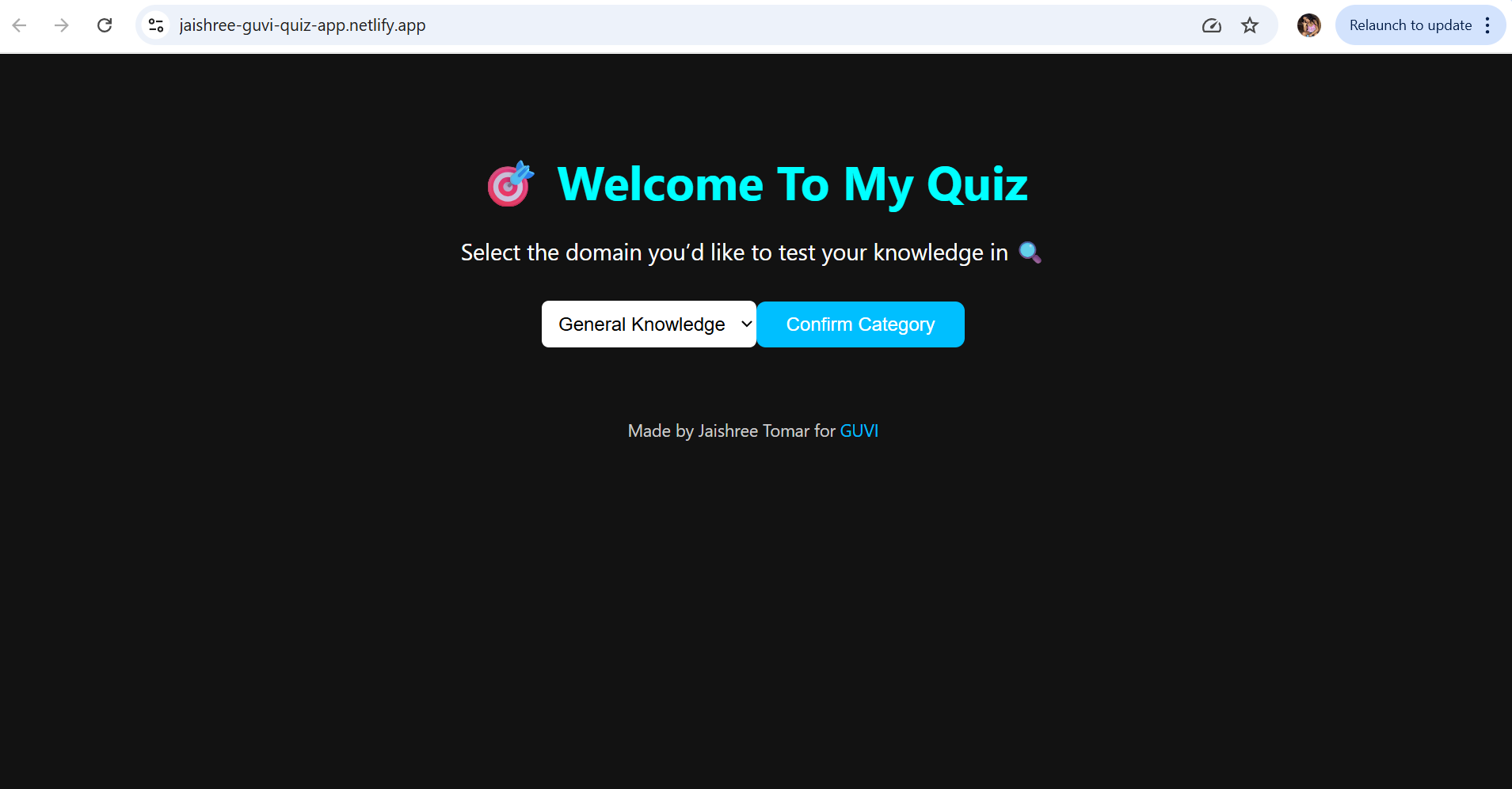
Building a Quiz App in ReactJS
Build a React Quiz App with category selection, random questions, and a live scorecard. Clean UI, no backend, and perfect for mastering React fundamentals.
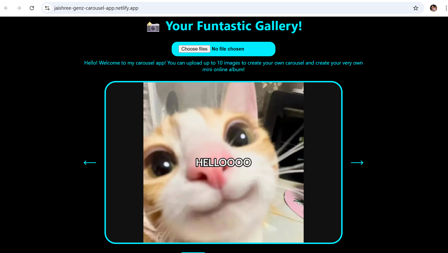
Building a GenZ Carousel App in React
Build a Gen-Z Image Carousel App with uploads, animated slides, and thumbnail navigation. No backend needed—perfect for learning React, hooks, and styling basics.
ReactJS Projects Handbook
Learn ReactJS by building projects that mirror real-world applications. Strengthen your skills with step-by-step guidance and hands-on coding experience.
Computer Networks Tutorial
A complete guide to computer networking, from fundamentals to protocols, routing, addressing, and real-world data communication.
Operating System Tutorial
Your complete guide to Operating Systems, from fundamentals to advanced topics like memory management, scheduling, threads, and deadlock handling.
DBMS and SQL Tutorial
A complete handbook to guide you through DBMS fundamentals and SQL mastery, perfect for building data-driven applications, managing data systems, or preparing for database roles.
Java Tutorial
Beginner-friendly Java handbook covering core concepts, OOP principles, and hands-on programming examples.
C Language Tutorial
A step-by-step C programming handbook for beginners. Understand C syntax, logic, memory, and hands-on coding to build solid programming foundations.
PHP Tutorial
Step-by-step PHP handbook for web developers. Master server-side scripting with practical code and concepts.

Android Tutorial
Beginner-friendly Android handbook covering app fundamentals, UI design, and hands-on development concepts.
Linux Guide Tutorial
A practical Linux handbook covering command-line basics, file management, and system operations.
Data Structures and Algorithms Tutorial
Learn core data structures and algorithms with practical examples to improve coding efficiency and problem-solving skills.
Computer Architecture
A beginner-friendly guide to computer architecture covering processors, memory, and system-level concepts.
HTML 5 References Tutorial
A handy HTML5 reference guide covering modern tags, attributes, and semantic elements.
Docker Tutorial
A hands-on Docker handbook covering containers, images, and modern application deployment basics.
GIT (Using Github) Tutorial
A hands-on Git and GitHub handbook for managing code, tracking changes, and collaborating on projects.

Go Language Tutorial
A beginner-friendly Go handbook covering core language concepts and modern backend programming.

GIT Guide
A practical Git guide covering version control basics, branching, and real project workflows.
CSS Tutorial
A beginner-friendly CSS handbook covering page styling, layouts, and responsive design basics.
Advanced Data Structures
A focused handbook covering advanced data structures for efficient and scalable problem solving.

Spring Framework Tutorial
A hands-on Spring Framework handbook covering core concepts and backend development fundamentals.

Spring Boot Tutorial
A practical Spring Boot handbook focused on building and running modern Java backend applications.
Kotlin Tutorial
A beginner-friendly Kotlin handbook covering modern language features and real-world development concepts.
Apache Cordova Tutorial
A hands-on Apache Cordova handbook for building cross-platform mobile apps with web technologies.
Python Tutorial
A beginner-friendly Python handbook covering core concepts and practical programming examples.
SASS-SCSS Tutorial
A hands-on SASS / SCSS handbook for writing clean, reusable, and scalable stylesheets.

MongoDB Tutorial
A hands-on MongoDB handbook covering NoSQL concepts and modern database operations.

Numpy Tutorial
A hands-on NumPy handbook for fast numerical computation and data manipulation using Python.
PL-SQL Tutorial
A hands-on PL/SQL handbook for writing procedural database programs and business logic.
Python Built-in Functions Tutorial
A handy reference guide to Python’s built-in functions for cleaner and faster coding.

Pandas Tutorial
A hands-on Pandas handbook for data manipulation, cleaning, and analysis using Python.

Elasticsearch Tutorial
A hands-on Elasticsearch handbook covering indexing, searching, and data analysis concepts.
Matplotlib Tutorial
A hands-on Matplotlib handbook for creating charts and visualizing data using Python.

Web Scraping Tutorial
A hands-on web scraping handbook for extracting and working with data from websites.
Networking with Python
A hands-on handbook for building network-enabled applications using Python.

Tkinter Tutorial
A hands-on Tkinter handbook for building desktop applications with Python.
Java Programs Tutorial
A hands-on Java programs handbook for practicing core concepts and problem-solving in Java.
Java Examples Tutorial
A hands-on Java examples handbook focused on logic building and practical coding.

Servlet Tutorial
A hands-on Java Servlet handbook for building server-side web applications.
JSP Tutorial
A hands-on JSP handbook for creating dynamic server-side web pages with Java.
Java Type Conversion Tutorial
A concise Java handbook explaining type conversion and casting with clear examples.
Java 8 Tutorial
A hands-on Java 8 handbook focused on modern language features and functional programming.
Java 9 Tutorial
A practical Java 9 handbook covering modules and platform enhancements.
Java 10 Tutorial
A focused Java 10 handbook covering language refinements and performance upgrades.
Java 11 Tutorial
A hands-on Java 11 handbook focused on modern APIs and long-term support features.
Java Util Library Tutorial
A hands-on Java Util library handbook covering essential utility classes and collections.
Building a Contact Us Form in ReactJS
Responsive ReactJS Contact Form with validation, error messages, and success animation.

Building a Age Calculator App Using ReactJS
Quickly find your exact age with this interactive ReactJS Age Calculator.
Movie Recommendation System Project Using Content-Based Filtering
Build a movie recommendation system that suggests similar movies using genre similarity and average ratings. A simple, practical ML project for beginners to understand real-world recommenders.
Recipe Finder App using ReactJS
Build a live Recipe Finder app using ReactJS. Search recipes, view details in modals, and handle state, events, and API data efficiently.

Sales Data Analysis Project for Beginners Using Data Science
Analyze sales data to find revenue trends, top products, quarterly patterns, and key customer insights. A beginner-friendly project for hands-on business data analysis in Python.
Student Performance Analysis Project for Beginners Using Data Science
Analyze student performance data to uncover attendance trends, study patterns, score improvements, and key exam factors. A beginner-friendly Python project for hands-on learning.

Word Counter Tool Using ReactJS
Learn to create a live Word & Character Counter using ReactJS, Tailwind CSS, and JavaScript. Practice state, events, and conditional rendering.
Customer Churn Prediction Project Using Classification Techniques
Analyze telecom customer data to predict churn, identify high-risk users, and uncover patterns in tenure, payments, and service usage. A beginner-friendly Python project for hands-on learning.
Basic Expense Tracker App using ReactJS
A simple ReactJS-based Expense Tracker App that helps users manage income, add expenses, and view real-time balance updates.

Simple Binary to Decimal Converter in React
A ReactJS tool that converts binary numbers into decimal form with instant validation and user-friendly input handling.
Real-Time Unit Converter in React
A ReactJS-based real-time converter that switches between units like length, weight, and temperature with instant results and swap functionality.

House Price Prediction Using Machine Learning (XGBoost)
Build a machine learning model that predicts house prices using housing characteristics and XGBoost Regression. A beginner-friendly project for learning real-world predictive analytics.
Weather Data Analysis and Visualization Using Python
Analyze weather data using Python and create visualizations to uncover temperature, humidity, and rainfall trends. A beginner-friendly Data Science project for learning practical data analysis.
Expandable Accordion Component using React
Learn to create an interactive React Accordion with toggle functionality and dynamic content display.

OTP Verification Component using React
Learn to build an interactive OTP Verification Component in React with auto focus, OTP validation, loading states, and resend functionality.
Cricket Data Analysis Using Python
Analyze IPL match data using Python to uncover player, team, and performance trends through data visualization. A beginner-friendly Data Science project for learning exploratory data analysis.
Credit Card Fraud Detection for Beginners using Data Science
Detect fraudulent credit card transactions using Logistic Regression and machine learning. Learn data preprocessing, classification, and model evaluation.
Deep learning Tutorial
A hands-on Deep Learning handbook covering neural networks, CNNs, RNNs, and modern AI architectures with practical examples.
Software Development Life Cycle Tutorial
A structured SDLC handbook covering software development phases, popular models, and real-world project workflows.
Stock Price Prediction for Beginners using Data Science
Predict future stock closing prices using historical market data and KNN Regression. Learn feature engineering, model optimization, and regression evaluation in this practical Data Science project.
Apache Kafka Tutorial
A hands-on Apache Kafka handbook covering topics, partitions, brokers, and real-time data streaming concepts.
Angular Tutorial
A hands-on Angular handbook covering components, services, routing, and building dynamic single-page web applications.

Django Tutorial
A hands-on Django handbook covering models, views, templates, and building full-featured web applications with Python.
Computer Programming Tutorial
A beginner-friendly programming handbook covering core coding concepts, logic building, and problem-solving fundamentals.
Tensorflow Tutorial
A hands-on TensorFlow handbook covering tensors, neural networks, and building deep learning models with Python.
Java OOPs Concepts Tutorial
A hands-on Java OOPs handbook covering classes, objects, inheritance, and the four pillars of object-oriented programming.
Building an Image Classification System Using CNN
Build an Image Classification System using TensorFlow and Keras. Learn image preprocessing, ANN, CNN, model evaluation, and image prediction through this beginner-friendly deep learning project.
News Recommendation System Using Machine Learning
Build a content-based News Recommendation System using Python, TF-IDF Vectorization, and Cosine Similarity to recommend relevant news articles through Machine Learning.
Fake Review Detection System using Machine Learning
Build a Fake Review Detection System using Python, TF-IDF Vectorization, and Logistic Regression to identify fake and genuine customer reviews through Machine Learning.
Product Feedback App Using Full Stack Development - Customer Review and Rating System
Build a complete Product Feedback App in React and learn modern frontend development through a practical, project-based approach.
Job Portal with Applicant Tracking System Using Full Stack Development
A Job Portal built with React JS — job seeker applications, employer dashboard, and reusable components.

(FalCon Store) A Modern React-Based E-Commerce App UI with Admin Dashboard
A React JS e-commerce project with a working cart, checkout flow, and admin panel to manage products and orders.
Student Management System using Python (Beginner-Friendly Project Guide)
A menu-driven Python project using SQLite to manage student records, attendance, and report cards.
HTML Tutorial - From Basics to Implementation
A complete HTML Tutorial covering every core concept, from basic tags to a fully built project with styling and interactivity.
Machine Learning Tutorial
This Machine Learning Tutorial covers theory, Python, algorithms, model evaluation, and a real project, built for learners at every level, from beginners to working professionals.
ReactJS Tutorial
Learn ReactJS from scratch and build interactive web applications with hands-on examples covering components, Hooks, routing, APIs, and performance optimization.

Hibernate Tutorial
A practical Hibernate Tutorial for Java developers. Learn ORM, entity mapping, relationships, HQL, caching and Spring Boot integration.

Data Analysis with Python Handbook
Learn to clean, analyze, and visualize data using Python. Go from the basics to advanced analytics with NumPy, Pandas, and real-world projects.

Artificial Intelligence Tutorial
Learn the different types of AI, how they work, their real-world applications, and how to choose the right AI approach through practical examples and activities.
Power BI Tutorial
Learn Power BI step by step, from data cleaning and modeling to DAX, interactive dashboards, and report publishing through practical projects for beginners.
R for Data Science
Master R programming, data manipulation, visualization, statistical analysis, and machine learning through practical examples and hands-on projects.
SQL for Data Science
A short, practical handbook with 21 lessons, from PostgreSQL setup and joins to window functions and using SQL with Python.

Data Analytics Tutorial
Learn the core skills of data analytics, how to turn raw data into insights, apply them to real business problems, and build job-ready skills through practical examples and exercises.